ENGI 3423 Probability and Statistics

Faculty of Engineering and Applied Science
2010 Fall

Solutions to Practice Questions
Term Test 1

[Descriptive Statistics and Elementary Probability]


  1. The actual time, in hours, to failure of a prototype mechanical component in a turbine, is measured on fifty occasions in an experiment.   The raw results are displayed here, sorted into increasing order:

    11 14 20 23 31 36 39 44 47 50
    59 61 65 67 68 71 74 76 78 79
    81 84 85 89 91 93 96 99101104
    105105112118123 136139141148158
    161168184206248 263289322388513

    The summary statistics include
              n = 50,   Sum(x) = 5963 ,   Sum(x^2) = 1176795


    1. From the summary statistics, calculate the sample mean and sample standard deviation for these data.
      xBar = 5963/50 = 119.26 ,
    s^2 = (50*1176795 - 5963^2)/(50*49) =  9503.01... ,
    s = 97.48 (4 s.f.)

    2. From the histogram below, identify the modal class.
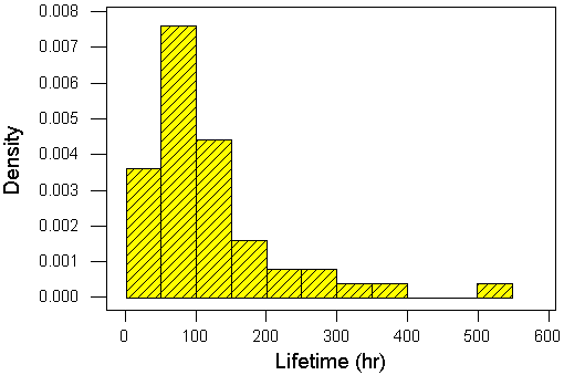
      histogram of lifetime data
      The modal class has the bar with the greatest area.
      With all class widths equal, that is also the tallest bar.
      Obviously, the modal class is
        [50, 100) hours  

    3. What evidence is there, from the histogram, for skewness?
      The right tail is considerably thicker and longer than the left tail.
      There is strong evidence for a substantial positive skew.

    4. Use the histogram only, to estimate the number of components in the sample, whose lifetimes are less than 50 hours.
      Lifetimes less than 50 hours are represented by the first class (and therefore the first bar) in the histogram.
      Relative frequency   =   area of bar   =   (width) × (height) .
      The width of the bar is 50 hours.
      The height seems to be between 0.0036/hr and 0.0037/hr.
      The relative frequency is therefore between 18% and 18.5%.
      The frequency = (relative frequency) × n   =   (between 18% and 18.5%)×50   =   9 to 9.25 .
      But the frequency must be a whole number.   Therefore
        n(T < 50 hours)   =   9  

    5. A stem-and-leaf diagram for these data is
          9    0 112233344
        (19)   0 5566667777788889999
         22    1 00001123344
         11    1 5668
          7    2 04
          5    2 68
          3    3 2
          2    3 8
          1    4 
          1    4 
          1    5 1
      
      Use this stem-and-leaf diagram to construct a frequency (and cumulative frequency) table and hence find the median class.
        Lifetime Frequency Cum. Freq.
        [0, 50) 9 9
        [50, 100) 1928
        [100, 150)1139
        [150, 100) 443
        [200, 250) 245
        [250, 300) 247
        [300, 350) 148
        [350, 400) 149
        [400, 450) 049
        [450, 500) 049
        [500, 550) 150

      The median class is where the 25th and 26th values fall, which is clearly the class [50, 100) .
      [In a stem-and-leaf diagram, the median class is very easy to find.   Seek the row where the cumulative frequency in the first column is replaced by a frequency in brackets, in this case (19).]

    6. Find the median value from the original data.
      From the stem-and-leaf diagram, one can identify the 25th and 26th values as being between 90 and 99 inclusive.   From the raw data, the median is (91 + 93) / 2 = 92.

    7. The asterisk in the boxplot below denotes the location of the sample mean.
      Describe the evidence for skewness that you can see in the boxplot.
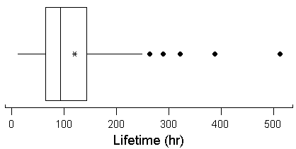
      boxplot of lifetime data
      All of the following provide very strong evidence for a substantial positive skew in the data:
      • The right whisker is much longer than the left whisker.
      • The upper quartile is much further away from the median than the lower quartile.
      • The mean is greater than the median.
      • There are five outliers, all greater than the median.

    8. List all the outliers.
      The outliers are the five largest values in the data set.
      They are
        263, 289, 322, 388, 513  
      The first three are mild outliers, the latter two are extreme outliers.
      [The upper outer fence is at
      (upper quartile) + 3×(inter-quartile range) = 142.75 + 3×78.75 = 379.]

  1. A box contains 11 different [distinguishable] gear wheels.   In how many ways can 3 gear wheels be drawn from the box, if they are drawn

    1. with replacement (order of selection matters)?
      nr = 113 = 1 331

    2. without replacement (order of selection matters)?
      11P3  =  11×10×9  =  990

    3. without replacement (order of selection is irrelevant)?
      11C3  =  11P3 / (3×2×1)  =  165


  1. Each of 12 refrigerators of a certain type has been returned to a distributor because of the presence of a high-pitched oscillating noise when the refrigerator is running.   Suppose that four of these 12 have defective compressors and the other eight have less serious problems.   If they are examined in random order, let X = the number among the first six examined that have a defective compressor.   Compute

    1. P[ X = 1]

      [Note:   The probability distribution here is hypergeometric.   It is not binomial, because the refrigerators are being sampled without replacement from a small population.   Knowledge of the hypergeometric probability distribution is not essential for the correct solution of this problem.]

      The population contains 4 defective compressors, of which x are in the random sample
      and
      the population contains 8 good compressors, of which 6 – x are in the random sample.
      From the total population of 12 compressors, a random sample of total size 6 is being drawn.

      The probability distribution is
              p(x) = 4Cx × 8C6 – x / 12C6   ,     (x = 0, 1, 2, 3, 4 only).

      Therefore   P[ X = 1] = 4C1 × 8C6 – 1 / 12C6   = ... = 4 × 56 / 924
      = 8 / 33 = .2424


    2. P[ X > 4]

      P[ X > 4] = P[ X = 4] = 4C4 × 8C6 – 4 / 12C6   = ... = 1 × 28 / 924
      = 1 / 33 = .0303


    3. P[1 < X < 3]

      Given the previous work in this question, it is easier to evaluate the probability via the complementary event (which is {X = 0 union X = 4}).

      P[1 < X < 3] = 1 – P[X = 0] – P[X = 4]
      = 1 – 4C0 × 8C6 – 0 / 12C6 – 1 / 33
      = 1 – 1 × 28 / 924 – 1 / 33 = 1 – 2 / 33
      = 31 / 33 = .9394


    [Omitted calculation details:     4C0 = 4C4 = 1 ;   4C1 = 4 ;
    Calculation of 8C5 = 56, 8C2 = 28 and 12C6 = 924


  1. A mathematics professor teaches both morning and afternoon sections of a course.
    Let A = {the professor gives a bad morning lecture}
    and B = {the professor gives a bad afternoon lecture}.
    If P[A] = .3 ,   P[B] = .2   and P[A and B] = .1 ,   then calculate the following probabilities (a Venn diagram might help) and calculate the equivalent odds:

    1.   P[B | A]

      First note that the odds r that are equivalent to a probability p are given by   r = p / (1-p)

      P[B | A] = P[A B] / P[A] = .1 / .3
      = 1 / 3 = .3333     implies r = 1:2 on = 2:1 against.


    2.   P[~B | A]

      P[A logical and ~B] = P[A] – P[A logical and B] = .3 – .1 = .2   (total probability law)
      P[~B | A] = P[~B A] / P[A] = .2 / .3
      = 2 / 3 = .6667     implies r = 2:1 on.

      OR

      Total probability law (and part (a))     implies
      P[~B | A]   =   1 – P[B | A]   =   1 – 1/3   =   2 / 3     implies r = 2:1 on.


    3.   P[B | ~A]

      P[~A logical and B] = P[B] – P[A logical and B] = .2 – .1 = .1
      and   P[~A] = 1 – P[A] = .7
      P[B | ~A] = P[B ~A] / P[~A] = .1 / .7
      = 1 / 7 = .1429     implies r = 1:6 on = 6:1 against.


    4.   P[~B | ~A]

      P[~A logical and ~B] = P[~(A logical or B)] = 1 – P[A logical or B] = 1 – P[A] – P[B] + P[~A logical and B]
      = 1 – .3 – .2 + .1 = .6
      P[~B | ~A] = P[~B ~A] / P[~A] = .6 / .7
      = 6 / 7 = .8571     implies r = 6:1 on.

      OR

      Total probability law (and part (c))     implies
      P[~B | ~A]   =   1 – P[B | ~A]   =   1 – 1/7   =   6 / 7     implies r = 6:1 on.


    5. If, at the conclusion of the afternoon class, the professor is heard to mutter “what a rotten lecture”, then what is the probability that the morning lecture was also bad?


      P[A | B] = P[A B] / P[B] = .1 / .2
      = 1 / 2 = .5000     implies r = 1:1 = even odds.


    1. An engineer states that the odds of a prototype microchip surviving a current of 3 µA for 2 hours is “4 to 1 against”.   What is the engineer’s probability for this event?


      Odds of “4 to 1 against” means “1 to 4 on”.
      r = 1:4     Þ     probability   p = r / (r + 1)   =   (1/4) / (5/4)   =   1/5.


    2. The event E is defined to be
            “the score on a roll of a fair die is either a prime number or 1”.
      Calculate the odds on E, expressed as a ratio reduced to its lowest terms.

      E = { 1, 2, 3, 5 }
      Þ     P[E] = 4/6 = 2/3
      Þ     Odds on E are   r = p / (1 - p) = (2/3) / (1/3)
      r = 2:1 on   (or 1:2 against).


  1. Odds vs. Bookies’ Odds

    In a five horse race, you can place a bet of $180pi and if event   Ei (= horse i wins) occurs, then you win the bookie’s stake of $180.   The stake is the same for every horse.
    The bookie quotes odds of

    r1 = 5 to 4 on, r2 = 3 to 1 against, r3 = 7 to 2 against,
    r4 = 17 to 1 against

    and r5 = 17 to 1 against

    1. Are these odds fair?   Justify your answer by determining whether or not the probabilities associated with these odds are coherent.

    2. r1 = 5/4   Þ   p1 = (5/4) / (9/4) = 5/9
      r2 = 1/3   Þ   p2 = (1/3) / (4/3) = 1/4
      r3 = 2/7   Þ   p3 = (2/7) / (9/7) = 2/9
      r4 = r5 = 1/17   Þ   p4 = p5 = (1/17) / (18/17) = 1/18

      The sum of these five probabilities is 41/36 which is not equal to 1.
      The probabilities are therefore incoherent.

      Answer:   NO


    3. What is the bookie’s guaranteed profit if you place one bet on each of all five horses?

      The bookie’s net gain if horse h wins is
      gh = (3 pi si) - sh
          = s ((3 pi) - 1)
      (because the bookie’s stake is the same for all five horses)
          = 180 × (41 - 36) / 36
      The guaranteed profit is   $25.


  1. An electronic [or structural] system consists of five electronic [or structural] components arranged as follows:
    Circuit A to R1 to 
 [parallel: (series {parallel R2, R4}, R5), R3] to B

    Each component is operative or fails under load.   The probability of failure for each individual component is .01.   The entire assembly fails only if the path from A to B is broken.   The sample space S consists of all possible arrangements of operative and inoperative components.

    1. Show that n(S) = 32.

      There are 5 components, each of which can be operative or non-operative (two possible states).
      Therefore   n(S) = 25 = 32.


    Let E1 = "the assembly is operative";
          E2 = "R2 has failed but the assembly is operative";
          E3 = "R3 has failed but the assembly is operative";
    and F = "the assembly has failed".

    1. Are E1 and E2 mutually exclusive?

      NO.

      E2 occurs if components 1 and 3 are operative and component 2 fails, (regardless of the state of the other two components).   Thus events E1 and E2 can both occur.   The two events are therefore compatible.


    2. Are E1 and E3 mutually exclusive?

      NO.

      E3 occurs if components 1, 5 and at least one of 2 and 4 are operative and component 3 fails.   Thus events E1 and E3 can both occur.   The two events are therefore compatible.


    3. Are E2 and E3 mutually exclusive?

      NO.

      The assembly can be operative with only components 1, 4 and 5 operative (so that components 2 and 3 have failed).   This configuration is part of both events E2 and E3.   Events E2 and E3 are therefore compatible.


    4. Write down all the sample points in the event F, (that is, list all arrangements of operative and inoperative components that lead to the failure of the entire assembly).   Hence find n(F).

      Let   { 1 2 5 }   represent the sample point "only components 1, 2 and 5 are operative, the other components have failed".   Then the sample points in the event F are:

               {  }
               { 1 }   { 1 2 }  { 1 2 4 } 
                       { 1 4 }
                       { 1 5 } 
               { 2 }   { 2 3 }  { 2 3 4 }  { 2 3 5 }  { 2 3 4 5 }
                       { 2 4 }  { 2 4 5 } 
                       { 2 5 }
               { 3 }   { 3 4 }  { 3 4 5 }
                       { 3 5 }
               { 4 }   { 4 5 }
               { 5 }
      

      Therefore n(F) = 21.

      or

      It is easier to list the ways in which the assembly is operative (event ~F), because that event can occur only if component 1 is operative:

                   { 1 2 3 }  { 1 2 3 4 }  { 1 2 3 5 }  { 1 2 3 4 5 } 
                   { 1 2 5 }  { 1 2 4 5 }
          { 1 3 }  { 1 3 4 }  { 1 3 4 5 }
                   { 1 3 5 }
                   { 1 4 5 }
      

      Thus n(~F) = 11     Þ   n(F) = 32 - 11 = 21.


    5. Are the sample points in the event F equally likely?

      NO.

      For any one arrangement (such as { 1 3 5 }) with exactly three operative components, the probability of that arrangement is (.99)3×(.01)2 = .0000970299,   while for any one arrangement (such as { 1 3 }) with exactly two operative components, the probability of that arrangement is (.99)2×(.01)3 = .0000009801.
      The sample points are, therefore, not all equally likely.


    6. What is the probability that the assembly fails?
      [You may assume that component failures are independent of each other]

      Use the second solution to part (e) above to group the sample points of ~F into subgroups of equally likely sample points:

      Exactly two operative (probability for each point = (.99)2×(.01)3 = .00000098010):
        { 1 3 } only.
      n(two operative) = 1
      Þ   P[two operative and assembly operative] = .00000098010

      Exactly three operative (probability for each point = (.99)3×(.01)2 = .0000970299):
        { 1 2 3 }, { 1 2 5 }, { 1 3 4 }, { 1 3 5 }, { 1 4 5 } .
      n(three operative) = 5
      Þ   P[three operative and assembly operative] = .0004851495

      Exactly four operative (probability for each point = (.99)4×(.01)1 = .0096059601):
        { 1 2 3 4 }, { 1 2 3 5 }, { 1 2 4 5 }, { 1 3 4 5 } .
      n(four operative) = 4
      Þ   P[four operative and assembly operative] = .0384238404

      All five operative (probability for each point = (.99)5×(.01)0 = .95099005):
        { 1 2 3 4 5 } only.
      n(five operative) = 1
      Þ   P[five operative and assembly operative] = .95099005

      Therefore   P[assembly fails] = 1 - P[assembly operative]
      = 1 - (.00000098010 + .0004851495 + .0384238404 + .95099005)
      = .0101000   (correct to 6 significant figures).


  1. There are seven candidates in an election for three officers on the executive committee of a club.   In how many distinct ways can the voting members of the club fill the three vacancies if

    1. the three officer positions are identical (for example, they are all committee members without specific office);

      The same person cannot be elected to more than one position at the same time
      ®   sampling without replacement.

      The three positions are identical   ®   order of selection is irrelevant
        ®   combinations;   n = 7,   r = 3 .
      7C3 = 7! / (3! 4!) = (7×6×5) / (3×2×1) =

        35  


    2. the three officer positions are distinct (for example, the person with the most votes becomes president and the runner-up becomes vice president);

      The three positions are distinct   ®   order of selection matters
        ®   permutations;   n = 7,   r = 3 .
      7P3 = 7! / 4! = (7×6×5) =

        210  


  1. A certain rare disease is known to occur in 1% of the population.
    A diagnostic test exists for this disease, but the test is not perfect.
    If a person has the disease, then the test will [correctly] detect the disease 98% of the time.
    If a person does not have the disease, then the test will [incorrectly] claim a detection of the disease 10% of the time.

    Given a positive test result [implying that the person has the disease], what are the odds that the test result is correct, [the person really does have the disease]?


    Let   D   =   the event “the person really does have the disease”
    and   T   =   the event “the test indicates that the person has the disease”
    then     P[D] = .01 ,     P[T | D] = .98 ,   and   P[T | ~D] = .10
    The number P[D | T] is required.

    By Bayes’ theorem,
    P[D|T]  =  P[T|D] P[D] / P[T]
    implies P[D | T] = 98/1088 = 49/544     implies r [D | T] = 98/990 = 49/495   or

      495 : 49 against  

    [The following tree diagram may be used instead.]
    [tree diagram]


  1. Adam Ant is determined to return to his home I from his Aunt’s house A over the lattice of twigs shown below.

               A ---- B ---- C
               |      |      |
               |      |      |
               D ---- E ---- F
               |      |      |
               |      |      |
               G ---- H ---- I
    

    Being only a young ant, he can only move south (down the page) or east (right) at each junction.   Where there is a choice, Adam is equally likely to choose each of the two twigs.

    1. Write down the complete list of outcomes.
      (For example, one of the possible outcomes is the path ABEFI).
    2. Let X represent the number of junctions along the path at which Adam has a choice of twig.   Write down the complete set of possible values of X.

      Two choices exist at each of the points A B D E .

      Path X
      ABCFI 2
      ABEFI 3
      ABEHI 3
      ADEFI 3
      ADEHI 3
      ADGHI 2

      The set of possible values of X is thus

        { 2, 3 }  


    3. For each possible value of X, find the probability that that value of X occurs.
      [Be careful:   P[X = 2] is not 1/3 !]

      The six paths above are not equally likely!
      On any path, the probability of reaching the next named point from any of A B D E is 1/2.   The probability is 1 (absolutely certain) otherwise.   By the definition of X, each path has exactly X such decision points and the decisions are all independent of each other.   Therefore, for each of the six possible paths, the probability that that path is taken is (1/2)X.

      P[X = x] = (number of paths) × (probability for a path)
      P[X = 2] = 2 × (1/2)2 = 2/4 = 1/2
      P[X = 3] = 4 × (1/2)3 = 4/8 = 1/2


Also see the Term Tests from the years 2008, 2007 and 2006.


Index of Assignment Solutions [Return to the index of assignment solutions.]
Back to previous page [Return to your previous page.]

Created 1998 09 04 and most recently modified 2010 07 30.