ENGI 3423 Probability and Statistics

Faculty of Engineering and Applied Science
2010 Fall


Additional Exercises

[Topics after Test 2]

[Note:   The "Symbol" font is used in several places in these solutions.
Some solutions will not display correctly unless the "Symbol" font is installed on your computer.
Click here to download the "Symbol" font.]


  1. A production process gives components whose strengths are normally distributed with a mean of 400 N and a standard deviation of 11.5 N.   A modification is made to the process which cannot reduce but may increase the mean strength.   It may also change the variance.   The strengths of nine randomly selected components from the modified process, in Newtons, are:

     396   402   409   409   414   398   394   436   418

    Test, at a five per cent level of significance, the hypothesis that the mean strength has not increased.


    Let   X = component strength (N)
    X ~ N(µ, σ2)

    Test     null hypothesis: µ = 400     vs.     alternative hypothesis: µ > 400       at   α = .05
    σ2 is unknown for the new process.

    Data:
    n = 9 åx = 3676 åx2= 1502838 a = 0.05
    implies xBar = 408.444... s^2 = 12566/72 = 174.527... s = 13.21089617

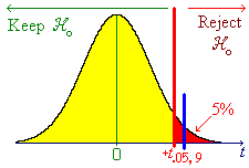
    Method 1

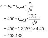
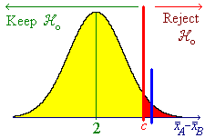
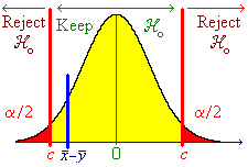
    [Graph showing rejection region]     c = muo + t*s/sqrt{n} = 400 + 1.85*4.40 = 408.188...

    xBar = 408.4... > c
    \ Reject null hypothesis in favour of alternative hypothesis at a = 0.05

    OR

    Method 2

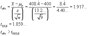
    t = (xBar - muo) / (s/sqrt{n})
  = 8.444 / 4.40  =  1.917
tc = 1.859 ;   tobs > tc
    \ Reject null hypothesis.

    OR

    Method 3

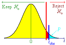
    From t-tables,   t.05, 8 = 1.859...   and   t.025,8 = 2.306...
    .025 < P[T>tobs] < .05     and     a = .05
    [From appropriate software,   P[T>tobs] = .045 < a]
    \ Reject null hypothesis.

    OR

    Confidence Interval Method

    c = xBar - t*s/sqrt{n} = 408.4 - 1.85*4.40
     = 400.25...
    \ we are “95% sure that µ > 400.25...”.
    µ = 400 is not inside this CI.
    \ Reject null hypothesis.

    At a = 5%, there is sufficient evidence to conclude that

      there has been an increase in mean strength.  

    An Excel spreadsheet file and a Minitab project file are also available to illustrate this solution.


  1. A transport firm is very suspicious of the tyre company’s claim that the average lifetime of its tyres is at least 45,000 kilometres.   The transport company decides to check this claim by fitting forty of these tyres to its trucks, the tyres being a random sample.

    A mean lifetime of 44,164 km with a sample standard deviation of 2,106 km is observed.   What may the transport firm conclude about the claim at a level of significance of one per cent?


    The burden of proof is on the transport firm, (to disprove the tyre company’s claim).

    Test:
       null hypothesis: µ > 45000   (tyre company’s claim.)
    vs.
       alternative hypothesis: µ < 45000
    at   a = .01

    Data:
    n = 40 xBar = 44164 s = 2106

    Method 1

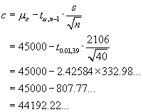
    [Graph showing rejection region] c = muo - t*s/sqrt{n} = 45000 - 2.425*332.98
         = 44192.22

    xBar = 44164 < c
    \ Reject null hypothesis in favour of alternative hypothesis.

    OR

    Method 2

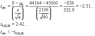
    tobs = (xBar - muo) / (s/sqrt{n})
  = (44164-45000)/(2106/sqrt{40}) = -2.51...
 t_.01,39 = 2.42
 tobs < -t_.01,39
    \ Reject null hypothesis.

    OR

    Method 3

    tobs = –2.51...
    From t-tables,   t.01, 39 = 2.425...   ,     P[T < tobs] < 0.01 (= a)
    [From appropriate software,   P[T < tobs] = 0.008... < a]
    \ Reject null hypothesis.

    OR

    Confidence Interval Method

    c = xBar + t*s/sqrt{n} = 44164 + 2.4*332.9
     = 44971.7...
    The one-sided 99% confidence interval estimate for µ is   µ < 44972 km.
    This CI does not include   µo = 45000
    \ Reject null hypothesis.

    \ the transport company does have sufficient evidence to dispute the tyre company’s claim.

    An Excel spreadsheet file is also available to illustrate this solution.

  1. A garage wants to know if a more expensive type of radial tyre has a tread life significantly more than 10,000 km beyond the tread life of a cheaper bias-ply tyre.   Only if this is the case will the garage invest in the more expensive type of tyre.   A random sample of forty tyres of each type is tested and the tread lives are measured.   The radial tyres have a mean tread life of 36,500 km with a standard deviation of 2,200 km, while the bias ply tyres have a mean tread life of 23,800 km with a standard deviation of 1,500 km.

    Based on these data, should the garage invest in the radial tyres?


    Let   XR = life of a randomly chosen radial tyre
    and   XB = life of a randomly chosen bias-ply tyre
    The burden of proof is on   µR > µB + 10000
    Free choice of a.   I choose a = 0.01

    Test:
        null hypothesis: µRµB = 10000 (or less)
    vs.
        alternative hypothesis: µRµB > 10000

    Data: nR = 40 xBarR = 36500 sR = 2200
    nB = 40 xBarB = 23800 sB = 1500

    An unpaired two-sample t-test is appropriate;
    measurements are on two different sets of individuals,
    (not pairs of measurements on the same one set of individuals).
    CLT  ==>  XbarR - XbarB ~ N(mu, sigma^2)

    Assume that sigmaR^2 = sigmaB^2 = sigma^2
    (The values of sR & sB lend some support to this assumption)
    [The sample sizes are just large enough to use the two sample z test instead, which does not require any assumption about the two population variances.   The eventual decision will be the same.]
    Pooled sample variance:
    sP^2  =  (39*2200^2 + 39*1500^2) / (39+39)
     = 3 545 000

    Method 1

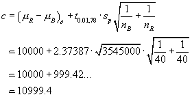
    [Graph of rejection region] c  =  (muR - muB)o  +  t_.01,78 * sP * sqrt{1/nB + 1/nR}
  = 10000 + 2.37... * sqrt{3545000 * (1/40 + 1/40)} 
        = 10999.4...

    [t.01, 78 has been approximated by t.01, 80 from the tables and is used in this solution.
    A reasonable level of precision would remain if t.01, 78 were to be approximated by t.01, ¥ = z.01.]

    xBarR - xBarB = 12700 > c
    \ Reject null hypothesis in favour of alternative hypothesis

      YES the garage should invest in the radial tyres.  

    OR

    Method 2

    t_obs  =  (xBarR - xBarB) - (muR - muB)o /
       (sP * sqrt{1/nR + 1/nB})
     =  (12700 - 10000) / (sqrt{3545000}*sqrt{2/40})
     =  6.41...
 t_.01,78  approx=  2.37...
 t_obs > t_.01,78
    \ Reject null hypothesis

    OR

    Method 3

    tobs = 6.41...
    From the t-tables,   P[T > tobs] << .005
    [From appropriate software,   P[T > tobs] » 5 × 10⁻⁹]
    \ Reject null hypothesis at any reasonable a.

    OR

    Confidence Interval Method

    The one sided CI for   µRµB has its boundary at:
    c  =  (xBarR - xBarB)  -  t_.01,78 * sP * sqrt{1/nR + 1/nB}
    =   12700 – 2.37...×421.0... =   11700.5...
    This 99% CI for   µRµB   is   µRµB > 11701 (to nearest km).
    The CI does not include 10000.
    \ Reject null hypothesis.

    An Excel spreadsheet file is also available to illustrate this solution.


  1. A particular type of motor is known to have an output torque whose range in normal operation follows a normal distribution.   Seven motors are chosen at random and are tested with the old and new methods of controlling the range of torque values.   The results of the tests are as follows:

    Motor: 1234 567
    New method: 5.253.164.436.12 5.752.216.01
    Old method: 7.836.227.468.83 8.195.648.88

    1. Justify your choice of method in (b) below.


      The data are pairs of measurements on a single set of individuals (the seven motors).
      \ the appropriate method is a

        paired two-sample t-test  

    2. Conduct an appropriate hypothesis test to determine whether there is sufficient evidence to conclude that the range of torques with the new method is at least 2 units less than with the old method.


      Let   X = torque (new method)
              Y = torque (old method)
      and   D = XY

      Test:
          null hypothesis: µD = –2
      vs.
          alternative hypothesis: µD < –2

      Free choice of a.   I choose a = 0.05

      Motor:1 23 45 67 Sum SSq
      x = New Method: 5.25 3.164.43 6.125.75 2.216.01   
      y = Old Method: 7.83 6.227.46 8.838.19 5.648.88   
      d = Difference: -2.58 -3.06 -3.03 -2.71 -2.44 -3.43 -2.87 -20.12 58.5004

      Data: n = 7 åd = –20.12 åd2 = 58.5004
      Þ xBar = -2.874285714 sD^2 = 4.6884/42  =  0.1116... sD = 0.334108622

      Method 1

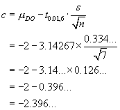
      [Graph of rejection region] c  =  muDo  -  t_.01,6 * sD/sqrt{n}
         =  -2 - 3.14*0.126  =  -2.396...

      xBarD  =  -2.87... < c
      \ Reject null hypothesis in favour of alternative hypothesis.

      OR

      Method 2

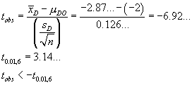
      t_obs  =  (xBarD - muDo) / (sD/sqrt{n})
     = -6.92...
 t_.01,6 = 3.14
 t_obs < -t_.01,6
      \ Reject null hypothesis.

      OR

      Method 3

      tobs = –6.92...
      Clearly P[T < –6.92] << .01
      [From software, P[T < –6.92] » 0.0002]
      \ Reject null hypothesis at any reasonable a.

      An Excel spreadsheet file is also available to illustrate this solution.


    3. Use the simple linear regression model on these data to find the equation of the line of best fit to these data.


      Note that the “line of best fit” depends on which variable is the predictor and which is the response.   The roles of X and Y are interchanged if the new method is the response, (which is the more natural assignment).

      Summary statistics (response = Y = old method):

      n = 7 åx = 32.93 åx2= 168.6941
      åxy = 260.7758 åy = 53.05 åy2= 411.3579

      n Sxx = 96.4738
n Sxy = 78.4941
n Syy = 65.2028
      beta1 = 0.813...  and  beta0 = 3.751...
      Therefore, (correct to 3 s.f. in each coefficient),

        y   =   0.814 x + 3.75  

      OR

      Summary statistics (response = Y = new method):

      n = 7 åx = 53.05 åx2= 411.3579
      åxy = 260.7758 åy = 32.93 åy2= 168.6941

      n Sxx   =   65.2028
      n Sxy   =   78.4941
      n Syy   =   96.4738
      beta1 = 1.203...  and  beta0 = -4.419...
      Therefore, (correct to 3 s.f. in each coefficient),

        y   =   1.20 x – 4.42  

      An Excel spreadsheet file is available to illustrate the first version of this solution.


    4. Find the coefficient of determination   R2   and use it to comment on your answer to part (a) above.


      Irrespective of which of old or new methods is the regressor,
      R^2 = Sxy^2 / (Sxx*Syy) = 0.97949...
      \     R 2 = 97.9%   (correct to 3 s.f.)

      Very high correlation     Þ     cannot use unpaired t-test.
      \ Choice in (a) is correct.

    A Minitab project file and a Minitab Report Pad RTF file are also available to illustrate this solution.


  1. A designer claims that a new type of hull increases the average sustained speed of a speedboat by more than 2 km/h over the average sustained speed of the existing hull design.   Random samples of speedboats of the two designs are tested and their sustained speeds (in km/h) are measured on a test course under identical water conditions:

    New design (xA):
         42    36    38    37    39    36
    
    Old design (xB):
     
         30    37    33    31    34   
    

    Conduct an appropriate hypothesis test at a level of significance of 5%.   Is there sufficient evidence to accept the designer’s claim?   What assumptions have you made?


    Calculation of summary statistics:
    New design
    speeds
    xA
    Old design
    speeds
    xB
    xA2 xB2
     
    42 30 1764  900
    36 37 1296 1369
    38 33 1444 1089
    37 31 1369  961
    39 34 1521 1156
    36 1296


    228 165 8690 5475

    nA = 6 nB = 5
    nA = 5 nB = 4
    xBarA = 38 xBarB = 33
    sA2 = 5.2 sB2 = 7.5

    The designer’s claim is that   µAµB > 2
    (which is where the burden of proof lies).
    Test
        null hypothesis: µAµB = 2
    vs.
        alternative hypothesis: µAµB > 2

    We assume that the two populations are independent, nearly normal and
    have a common population variance.

    Then E[XbarA-XbarB] = muA-muB and V[XbarA-XbarB] = sA^2/nA - sB^2/nB

    σ2 is unknown, so use the pooled sample variance

    sP^2 = (nuA sA^2 + nuB sB^2) / (nuA + nuB) = (5*5.2 + 4*7.5) / (5+4) = 56/9 = 6.2...

    The sample standard error is sqrt{sP^2 (1/nA + 1/nB)} = sqrt{6.2 (1/6 + 1/5)} = sqrt(2.2814...)

    The total number of degrees of freedom is   n = nA + nB = 9

    Method 1

    If null hypothesis is true, then   XbarAXbarB ~ N(2, σ 2)
    where σ 2 is approximated by 2.2814... .
    Upper tailed test.
    c = Do + ta, n × (s.e.) = 2 + t.050, 9 Ö 2.2814...
    = 2 + 1.833 × 1.5104... = 2 + 2.768...
    \   c = 4.768...
    xBarAxBarB = 38 – 33 = 5 > c

    \   reject Ho in favour of alternative hypothesis at a = .05 .


    OR

    Method 2


    t = ((xAbar-xBbar)-Do)/(s.e.)
 = ((38-33)-2)/sqrt(2.2814) = 1.986...

    tc = ta, n = t.050, 9 = 1.833

    tobs > tc
    \   reject Ho.


    OR

    Method 3

    As above,   tobs = 1.986 .
    t.050, 9 = 1.833   and   t.025, 9 = 2.262 .
    t.025, 9 > tobs > t.050, 9
    implies   .025 < p-value < .050
    But a = .05

    \   reject Ho.


      YES, we can accept the designer’s claim.  

    [Note:   if we had taken a = .01, then we would have reached the opposite conclusion,
    because the p-value is .039 (to 3 d.p.).]

    An Excel spreadsheet file and a Minitab project file are also available to illustrate this solution.


  1. The true mean tensile strength of a new type of lightweight cable is claimed to be more than 20 kN.   The distribution of actual strengths is known to be normal to a good approximation, with a standard deviation of 1.4 kN.   A random sample of five of the new cables has a mean of 21.5 kN

    1. Is there sufficient evidence to support the claim?


      Let   X = strength of a randomly chosen cable.           X ~ N(µ, σ 2)
      σ = 1.4 kN         n = 5         xBar = 21.5 kN

      Test:         null hypothesis: µ = 20      vs.     alternative hypothesis: µ > 20

      σ is known, therefore use z instead of t.
      Free choice of a.   I choose a = 0.01

      Method 1

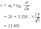
      c = muo + z_.01 * sigma/sqrt{n}
     = 20 + 2.32...*1.4/sqrt{5}
     = 21.456...
      xBar = 21.500 > c     (just barely)
      \ Reject null hypothesis in favour of alternative hypothesis at a = 0.01 (or any higher a)

      OR

      Method 2

      z_obs = (xBar - muo) / (sigma/sqrt{n})
     = (21.5 - 20) / (1.4/sqrt{5})
     = 2.39...
      z.01 = 2.32...
      zobs > z.01
      \ Reject null hypothesis.

      OR

      Method 3

      F(–2.39) » .008 < .01
      \ Reject null hypothesis.

      OR

      Confidence Interval Method

      c = xBar - z_.01 * sigma/sqrt{n}
     approx= 20.04
      The 99% CI for µ is   µ > 20.04 ,   which does not include µ = 20.
      \ Reject null hypothesis.

      An Excel spreadsheet file is also available to illustrate this solution.


    2. Now suppose that the standard deviation   sigma   is unknown and that the measured standard deviation of the random sample is s = 1.4 kN.   Is there sufficient evidence to support the claim?


      Now σ is not known and n = 5, therefore replace z by t.

      Method 1

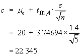
      c = muo + t_.01,4 * s/sqrt{n}
     = 20 + 3.74...*1.4/sqrt{5}
     = 22.345...
      xBar = 21.5 not> c
      \ do NOT reject null hypothesis at a = 0.01 .
      [If a = 0.05 were chosen, then
      c  =  20 + 2.13...*1.4/sqrt{5}  =  21.334 Þ opposite conclusion]

      OR

      Method 2

      t_obs  =  (xBar - muo) / (s/sqrt{n})
     = (21.5 - 20) / (1.4/sqrt{5})
     = 2.39...
      t.01, 4 = 3.74...
      tobs < t.01, 4
      \ do NOT reject null hypothesis at a = 0.01 .
      [t.05, 4 = 2.13...     implies tobs > t.05, 4         \ Reject null hypothesis at a = 0.05]

      OR

      Method 3

      t.05, 4 = 2.13...         tobs = 2.39...     and     t.01, 4 = 3.74...
      implies 0.01   <   P[T > tobs]   <   0.05
      \ do NOT reject null hypothesis at a = 0.01,
      [but do reject null hypothesis at a = 0.05]
      p-value (from software) is   P[T > tobs] = 0.037...

      OR

      Confidence Interval Method

      c  =  xBar - t_.01,4 * s/sqrt{n}
     = 21.5 - 3.74...*1.4/sqrt{5}
     = 19.154...
      The 99% one-sided CI for µ is   µ > 19.15 ,   which includes   µ = 20.
      \ do NOT reject null hypothesis.
      [The 95% CI for µ is   µ > 20.17 ,   which does not include µ = 20       \ Reject null hypothesis.]

      An Excel spreadsheet file is available to illustrate this solution, with a = 1%.
      An Excel spreadsheet file is also available for a = 5%


  1. Random samples are drawn from two independent populations, producing the following summary statistics:

    nX = 50  xBar = 643  sX = 26
nY = 90  yBar = 651  sY = 32

    Are these data consistent with the hypothesis that the two population means are equal?


    The burden of proof is on the alternative hypothesis that the two population means are not equal.   Therefore test
        null hypothesis: µXµY = 0     vs.     alternative hypothesis: µXµY ¹ 0

    From the question, the random quantities X and Y are independent, but we cannot assume equality of the variances.
    [In this course, we have not investigated how to test for equality of variances.   See section 9.5 of the Devore textbook.   As it happens, the data are consistent with sX2 = sY2.]

    The Central Limit Theorem leads to
    Xbar ~ N(mu_X, sigma_X^2 / n_X),
     Ybar ~ N(mu_Y, sigma_Y^2 / n_Y)
    and
    Xbar - Ybar ~ N(mu_X - mu_Y, sigma_X^2/50 + sigma_Y^2/90)

    Approximate the unknown   sX2   and   sY2   by the point estimates   sX2   and   sY2   respectively,
    and we may approximate ta, n by za.

    If   Ho is true, then, to an acceptable approximation,
    Xbar - Ybar ~ N(0, 26^2/50 + 32^2/90) = N(0, 24.897)

    Method 1:

    c = Delta_o + z_alpha/2 * sqrt{sX^2/nX + sY^2/nY}
    = 0 + 1.960*sqrt{24.897}  (alpha=5%)
             = 0 + 2.576*sqrt{24.897}  (alpha=1%)
    The boundaries of the rejection region are
    symmetric about   Do (= 0).
        implies cL = – cU = – c .
    The boundaries of the rejection region are at
    c = 9.780  (alpha=5%)
              = 12.854   (alpha=1%)
    xBar - yBar = 643 - 651 = -8
    -c < xBar - yBar < +c

    Therefore do not reject Ho.


    OR

    Method 2:


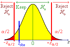
    z = ((xBar - yBar) - Delta_o) / sqrt{sX^2/nX + sY^2/nY}
             = ((643-651)-0) / sqrt{24.897}
        implies zobs = –1.603...
    a = 5%     implies zc = z.025 = 1.960
    a = 1%     implies zc = z.005 = 2.576

    In both cases,   | zobs | < zc, so
    do not reject Ho.

    OR

    Method 3:

    zobs = –1.603... (as in method 2 above).

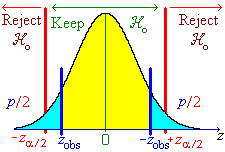
    The p-value   =   P[| Z | > | zobs |]   =   2 P[ Z < –1.603...]
    » 2 F(–1.60) » 2 × .0548 » .110 > .10

    Therefore do not reject Ho at any reasonable value of a.


    Answer:

      YES, these data ARE consistent with equal population means,  
    (although the p-value suggests that the agreement is not all that close).

    [See also the Excel spreadsheet file for this question.]

    [Note:   If a common variance had been assumed, then   sX2   and   sY2   would have been replaced by the pooled sample variance   sP2 = 124260/138.
    More precise estimates of the boundaries of the rejection region could have been obtained by using ta, n in place of za .
    With both changes in place, the boundaries of the rejection region for a = 5% would have moved out from ±9.78 to ±10.50.
    t.025, 138 » 1.98.
    The decision to retain Ho at any reasonable value of a is unchanged.]


  1. A study of company performance in two nearby cities was conducted to test for any significant difference between the companies in those cities.   A random sample of ten companies in city A had a sample mean performance index of 74.3 with a standard deviation of 3.2 .   A random sample of ten companies in city B had a sample mean performance index of 73.2 with a standard deviation of 2.9 .

    Is there a significant difference in company performance index between these two cities?   State carefully your assumptions and your hypotheses.


    We are dealing with two different sets of individuals, (the two sets of companies), the performances of which can be assumed to be independent of each other.   The sample variances are close enough to each other to support the assumption that the population variances are equal.   One further assumption (that is needed because of the small sample sizes) is that the performances are normally distributed to a fair approximation.

    We will therefore conduct an

      unpaired two sample t-test.  

    XA ~ N(µA, s2) ,     XB ~ N(µB, s2)

    Summary statistics:

    nA = 10 , xBarA = 74.3 , sA = 3.2
    nB = 10 , xBarB = 73.2 , sA = 2.9
    nA = nB = n – 1 = 9

    Test   null hypothesis : µAµB = 0     vs.     alternative hypothesis : µAµB ¹ 0

    Pooled sample variance:
    sp^2  =  (9*(3.2)^2 + 9*(2.9)^2) / (9 + 9)
     = 9.325
    Standard error:
    s.e.  =  sqrt{sp^2 * (1/nA + 1/nB)}
     =  sqrt{9.325 * 2/10}  =  sqrt{1.865}
    = 1.365 65...

    Total number of degrees of freedom = n = 18.

    We have a free choice of a.
    Even with an unusually large choice for a of 10%:

    Method 1

    c = Do ± ta/2, n × (standard error)
     = 0 ± 1.734 × Ö(1.865)
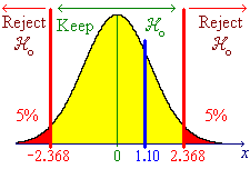
      = ± 2.368...
    xBarAxBarB = 74.3 – 73.2 = 1.100
    | 1.1 | < |c|
    Therefore do not reject null hypothesis .

    [If a = .05 is chosen, then c = ±2.869
    and
    if a = .01 is chosen, then c = ±3.930
    ® same result.]

    Two tailed rejection region graph

    OR

    Method 2

    tobs = ((xBarA - xBarB) - Delta_o) / (s.e.)
 = (74.3 - 73.2 - 0) / sqrt{1.865}  =  1.100 / 1.365... = 0.805...
    ta/2, n = t.05, 18 = 1.73...   [or t.025, 18 = 2.10... or t.005, 18 = 2.87...]
    |t| < ta/2, n
    t is nowhere near the rejection region.
    [A computer package will show that the p-value exceeds .40 !]
    Therefore do not reject null hypothesis.

      There is no significant difference in performance index between the two cities.  

    [See also the associated Excel file.]


  1. A study was conducted to analyze the relationship between advertising expenditure and sales.   The following data were recorded:

    X Y
      Advertising ($)     Sales ($)  
    20 310
    24 340
    30 400
    32 420
    35 490

    Assume a simple linear regression between sales Y and advertising X.   Calculate the coefficients β0 and β1 of the line of best fit to these data and estimate the sales when $28 are spent on advertising.

    Is there a significant linear association between Y and X?


    Extending the table:

          x         y       x2     x y     y2  
     20 310 400 6200 96100
     24 340 576 8160 115600
     30 400 900 12000 160000
     32 420 1024 13440 176400
     35 490 1225 17150 240100
    Sum:141 1960 4125 56950     788200    

      n Sxx = n å x2 – (å x)2    
        = 5 × 4125 – (141)2
        = 20625 – 19881
        = 744
      n Sxy = n å xy – (å x å y)
        = 5 × 56950 – 141 × 1960    
        = 284750 – 276360
        = 8390
      n Syy = n å y2 – (å y)2
        = 5 × 788200 – (1960)2
        = 3941000 – 3841600
        = 99400

    beta1 = Sxy/Sxx = 8390/744 = 11.276 881 72...

    beta0 = (Sumy - beta1*Sumx) / n = ... = 73.991 935 6...

    The regression line (to 4 s.f.) is  

      y = 11.28 x + 73.99  

    x = 28     implies y = 11.277... × 28 + 73.992...   =   389.744 623 7...

      When $28 is spent on advertising, we predict $390 of sales  

    (correct to the nearest dollar).


    There are many choices of method for an hypothesis test for linear association.
    Test null hypothesis : r = 0 vs. alternative hypothesis : r ¹ 0 ,
    or, equivalently,
    test null hypothesis : b1 = 0 vs. alternative hypothesis : b1 ¹ 0 .

    r^2 = Sxy^2 / (Sxx*Syy) = ... = .951...
    implies     just over 95% of all variation in   y   is explained by the linear regression.   The correlation (.975...) is very strong, (which suggests that there is a linear association), but the sample size is very small, so we should proceed with a formal hypothesis test.

    t  =  r * sqrt{n-2} / sqrt{1-r^2} = 7.700...


    or
    t  =  sqrt{Sxy^2 * (n-2) / (Sxx*Syy - Sxy^2)}
     =  sqrt{8390^2 * 3 /(744*99400 - 8390^2)}  = 7.700...


    or
    calculate the entries in the ANOVA table as follows:
    SSR = Sum(yHat - yBar)^2 = (nSxy)^2 / (n * nSxx)
     =  8390^2 / (5 * 744) = 18 922.607 52
    SST = Sum(y - yBar)^2 = Syy = nSyy / n = 19880
    SSE   =   SST     SSR   =   957.392 48
    MSR   =   SSR / nR   =   SSR   =   18 922.607 52
    MSE   =   SSE / nE   =   SSE / 3   =   319.130 826 6...
    f   =   MSR / MSE   =   59.294...

      d.f. SS MS f
        R         1         18 922.607 52...         18 922.607 52...         59.294...    
    E 3 957. 392 48... 319.130 826 6...
    T 4 19 880
    t   =   +Ö f   =   7.700...

    or
    sb^2  =  MSE / Sxx  =  5 * 319.13... / 744  =  2.144 696
    t  =  (betaHat1 - 0) / sb  =  11.27... / sqrt{2.144...}
     =  7.700...


    Compare the observed   t = 7.700...   to   t.005, 3 = 5.841...
    t > ta/2, 3 for any reasonable choice of a.
    [The p-value is less than .0046 .]
    Therefore reject null hypothesis in favour of alternative hypothesis     implies

      YES, there is a significant linear association between Y and X.  

    [See also the associated Excel and Minitab project files.]


  1. [Devore 6th ed., Ch. 12 p. 551 q. 73 - parts (b) & (c) are bonus questions only]

    The accompanying set of data is a subset of the data that appeared in the paper “Radial Tension Strength of Pipe and Other Curved Flexural Members” (J. Amer. Concrete Inst., 1980, pp. 33-39).   The variables are age of a pipe specimen (x in days) and load necessary to obtain a first crack (y in 1000 lb/ft).

    x 20 20 20 25 25 25 31 31 31
    y 11.45 10.42 11.14 10.84 11.17 10.54 9.47 9.19 9.54

    1. Calculate the equation of the estimated regression line.

      Summary statistics:

      n = 9 å x = 228 å y = 93.76
      å x2 = 5 958 å x y = 2 348.15 å y2 = 982.293 2

      implies
      n Sxx = 1 638 n Sxy = –243.93 n Syy = 49.701 2

      where   n Sxy = n å x yå x . å y   etc.

      beta1 = Sxy/Sxx = ... = 0.148 919 413...

      beta0 = (Sumy - beta1*Sumx) / n = ... = 14.190 402 92...

      The regression line (to 4 s.f.) is  

        y = 14.19 – 0.1489 x  

      A Minitab project file is also available to illustrate the solution to this part of this question.


    2. *   Suppose that a theoretical model suggests that the expected decrease in load associated with a 1 day increase in age is at most .10 (× 1000 lb/ft).   Do the data contradict this assertion?   State and test the appropriate hypotheses at significance level .05 .

      The slope b1 = the expected increase in load per day increase in age.
      The burden of proof is on showing that the [negative] slope is steeper than –0.10.

      Test null hypothesis : b1 = –0.10 vs. alternative hypothesis : b1 < –0.10 at a = .05.

      A chain of calculations follows.

      SSE = {(nSxx)(nSyy) - (nSxy)^2} / {n (nSxx)} = 1.486...
      MSE = SSE / (n-2) = 0.212...
      sb = sqrt{n MSE / (nSxx)} = 0.034...
      t = (beta1Hat - beta1o) / sb  =  -1.43...
      or, directly,
      t = {(nSxy) - beta1o*(nSxx)} *
 sqrt{(n-2) / [(nSxx)(nSyy) - (nSxy)^2]} = -1.43...

      But   t.05, 7 = –1.89... .

      Therefore do not reject null hypothesis.

        NO, the data do not contradict the assertion that b1 ³ –0.10.  

      Note   that the non-zero value of b1 in the null hypothesis renders the other versions of the t statistic incorrect.   They are based on the true [null] value of the slope being zero.


    3. *   For purposes of estimating the slope of the true regression line as accurately as possible, would it have been preferable to make a single observation at each of the ages 20, 21, 22, ..., 30 and 31?   Explain.

      For the original data, (nSxx) = 1638  ==>  Sum(x-xBar)^2  =  1638/9 = 182
      For the suggested new values of x ({20, 21, ..., 30, 31}),
      n = 12,     å x = 306,     å x2 = 7946
      implies     n Sxx = 1716     implies Sxx = 1716/12 = 143 .
      143 < 182   and we want Sum(x-xBar)^2 to be as large as possible because it appears in the denominator of the expression for the variance of the slope estimator, sb^2  =  MSE / Sum(x-xBar)^2.   A smaller value of   sb   leads to more precise estimates of the slope.

      [OR, the width of the confidence and prediction intervals contains a term (xo-xBar)^2 / Sum(x-xBar)^2.   These intervals are narrower when the denominator Sum(x-xBar)^2 is larger.]

      Therefore
        NO, the original data set is preferable,  
      despite its smaller sample size.

    4. Calculate an estimate of true average load to first crack when age is 28 days.   Your estimate should convey information regarding precision of estimation.

      95% Confidence interval for E[Y|28] :

      (b0 + b1*xo) +- t * sqrt{MSE*(1/n + n(xo-xBar)^2 / nSxx}
  = (14.19 + -0.148*28)
  +- 2.36 * sqrt{0.212*(1/9 + 9(28-228/9)^2 / 1638}
      = 10.020... ± 0.4223...

      Therefore the 95% confidence interval, to 2 d.p., is

        9.60 £ E[Y|28] £ 10.44  

      [See also the associated Excel file.]


  1. [Bonus question, to provide practice in the supplementary topic of type II error probabilities.]

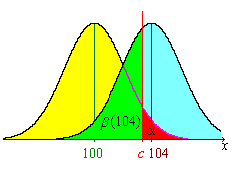
    Find the probability of committing a type II error when the true population mean is µ = 104 and an upper-tail hypothesis test is conducted at a level of significance of five per cent with a random sample of size 25 on the null hypothesis that µ = 100.   It is known that the population variance is 100.

    Repeat your calculation in the case when the level of significance of the hypothesis test is one per cent.


    null hypothesis : µ = 100     vs.     alternative hypothesis : µ > 100
    s2 = 100     implies s = 10
    n = 25     implies standard error = 2

    1. a = .05

      Use method 1.

      c   =   µo   +   za × (s / Ö(n))
          = 100 + 1.64... × 2
          = 103.290

      Probability of committing type II error
      when µ = 104   and   and a = .05   is
      beta(104) = P[Xbar < c | mu = 104]
      = P[Z < (c-104) / s.e.]
 = Phi((103.290 - 104) / 2)
      = F(-0.355)

      Graph for type II error

      implies
        b(104) = .361   (approx.)  

    2. a = .01

      Use method 1.
      c   =   µo   +   za × (s / Ö(n))
          =   100 + 2.32... × 2   =   104.652

      Probability of committing type II error when µ = 104 and a = .01
      beta(104) = P[Xbar < c | mu = 104]
      = P[Z < (c-104) / s.e.]
 = Phi((104.652 - 104) / 2)
      = F(+0.326)
      implies

        b(104) = .606   (approx.)  

    As expected, b increases as a decreases.


  1. [Bonus question, to provide practice in the supplementary topic of type II error probabilities.
    This question is a modification of Devore, 6th ed., Ch. 8.3, pp. 343-344, q. 38.]

    A university library ordinarily has a complete shelf inventory done once every year.   Because of new shelving rules instituted the previous year, the head librarian believes it may be possible to save money by postponing the inventory.   The librarian decides to select 800 books at random from the library’s collection and to have them searched in a preliminary manner.   If the evidence indicates strongly that the true proportion of misshelved or unlocatable books is less than .02, then the inventory will be postponed.

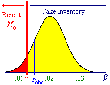
    1. Among the 800 books searched, 12 were misshelved or unlocatable.   Test the relevant hypotheses (at a level of significance of .05) and advise the librarian what to do.


      Let   p   represent the true proportion of books that are misshelved or unlocatable.
      Postpone the inventory if and only if there is strong evidence for   p < .02 .
      Therefore we need to test
          null hypothesis: p = .02     vs.     alternative hypothesis: p < .02

      n = 800
      a = .05   implies   za = 1.644...
      Observed sample proportion   p^ = 12 / 800 = .015

      Method 1

      c = p_o - z_alpha sqrt{p_o q_o / n}
  =  .02 - 1.645 sqrt{.02 x .98 / 800}

      = .02 – 0.008 142 334 5...
      = 0.011 857 665... = .0119 (to 4 d.p.)

      Graph of p.d.f. when p = .2

      Reject null hypothesis if and only if pHat < .0119
      But pHat = .0150 > c
      Therefore do not reject Ho

      In the remaining parts of this question, we need to know the value of c (the boundary of the rejection region when the null hypothesis is just barely true) in order to calculate the probability of rejecting (or not rejecting) the null hypothesis when the true value of p is something other than .02 . For this reason, we choose to use method 1 in part (a) of this question, rather than methods 2 or 3.

      [In method 2, the z score is –1.010, which is closer to z = 0 than
      the critical value of –1.645 .]
      [In method 3, P[Z < –1.010] = .1562 > a.]

      Whichever method we use, we decide to advise the librarian to
        proceed with the inventory.  

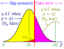
    2. If the true proportion of misshelved and lost books is actually .01, what is the probability that the inventory will be [unnecessarily] taken?


      Now we know that p = .01
      P^ ~ N(.01, (.01 x .99 / 800))

      P[inventory taken]
      = P[null hypothesis not rejected]
      P[P^ > c] = 1 - P[P^ < c]

      The boundary   c   of the rejection region
      is calculated on the basis that
      p = .02 .
      From method 1 in part (a),
      c = .011 857 665...

      Graph showing beta(.01)

      P[P^ < c] = Phi((c-.01)/sqrt{.01x.99/800}) 
 = Phi(.001857.../.003517...) = Phi(0.52807)

      Without linear interpolation,
      F(0.53) = .7019 = .702 (to 3 d.p.)
      implies
        P[inventory taken] = .298   (3 d.p.)  

      With linear interpolation,
      F(0.528 07) » F(0.52) + .807 × {F(0.53) - F(0.52)}
      = .6985 + .807 × (.7019 – .6985)
      = .6985 + .807 × .0034 = .6985 + .0027...
      = .7012 = .701 (to 3 d.p.)
      implies P[inventory taken] = .299.


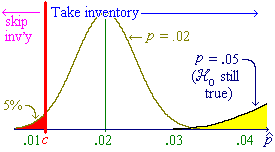
    3. If the true proportion is .05, what is the probability that the inventory will be postponed?


      Now we know that   p = .05 > .02 . P^ ~ N(.05, (.05 x .95 / 800))

      The correct decision now is to proceed with the inventory.

      The boundary   c   of the
      rejection region is
      calculated on the basis
      that   p = .02 .
      From method 1 in part (a),
      c = .011 857 665...

      P[inventory postponed]
      = P[null hypothesis rejected]

      Graph showing alpha(.05)

      = P[P^ < c] = Phi((c-.05)/sqrt{.05x.95/800})  
  = Phi(-.038142.../.007705...) = Phi(-4.95) = 0

        It is therefore very unlikely indeed that the inventory will be postponed.  

    4. What types of errors are the events described in parts (b) and (c) above?


      In (b), we are told that the true value of   p   is .01 .
      This is less than .02, so that the alternative hypothesis is true.
      The correct decision is to reject the null hypothesis; that is, to postpone the inventory.

      Taking the inventory = failure to reject the null hypothesis.
      Failure to reject the null hypothesis when it is false is a

        type II error.  


      In (c), we are told that the true value of   p   is .05 .
      This is greater than .02, so that the null hypothesis is true.
      The correct decision is to accept the null hypothesis; that is, to proceed with the inventory.

      Postponing the inventory = rejecting the null hypothesis.
      Rejecting the null hypothesis when it is true is a

        type I error.  

  1. [Bonus question only in 2008 Fall]
    [Devore 6th ed., Ch. 9.4 p. 398 q. 55]

    Two different types of alloy, A and B, have been used to manufacture experimental specimens of a small tension link to be used in a certain engineering application.   The ultimate strength (in ksi) of each specimen was determined and the results are summarized in the frequency distribution tabulated below.

    Alloy: A B
    26 - under 30 6 4
    30 - under 34 12 9
    34 - under 38 15 19
    38 - under 42 7 10
    sample sizes 40 42
    1. Compute a 95% confidence interval for the difference between the true proportions of all specimens of alloys A and B that have an ultimate strength of at least 34 ksi.


      Let   pA = proportion of alloy A that has ultimate strength ³ 34 ksi
      and   pB = proportion of alloy B that has ultimate strength ³ 34 ksi.

      Then pHat_A = 22/40 = .55 and pHat_B = 29/42 = .690 476 19...

      The point estimate of V[Phat_A - Phat_B] is pHat_A*qHat_A/n_A + pHat_B*qHat_B/n_B
      = (1*22*18)/(40*40*40) + (1*29*13)/(42*42*42)
      = 396/64000 + 377/74088 = 0.011 276 043

      A 95% CI for   pA – pB   is pHat_A - pHat_B +- z_.025*(s.e.)
      = (22/40 - 29/42) +- 1.960*sqrt{0.0112...} = –0.140 476 19 ± 0.208 129 882
      The CI is .349 < pA –   pB < +.068   (to 2 d.p.)


    2. Can you conclude that there is a significant difference between these two population proportions?


      NO because   pA = pB   is included in the 95% CI.
      [See also the Excel spreadsheet file for this question.]


  1. [Devore, ex. 12.4, q. 50 modified]

    An experiment to measure the macroscopic magnetic relaxation time in crystals (in microseconds, µs) as a function of the strength of the external biasing magnetic field (in kiloGauss, kG) yielded the following data (“An Optical Faraday Rotation Technique for the Determination of Magnetic Relaxation Times”, IEEE Trans. Magnetics, June 1968: 175-178, with data read from a graph that appeared in the article).

    x 11.012.515.217.2 19.020.822.024.2 25.327.029.0
    y 187225305318 367365400435 450506558

    The summary statistics are:
            n = 11 , sum x = 223.2 , sum y = 4116
sum x^2 = 4877.50 , sum xy = 90,096.1 , sum y^2 = 1,666,782

    1. Fit the simple linear regression model to these data.

      nSxx = 3834.26 ,  nSxy = 72365.9 ,  nSyy = 1393146
      slope = 18.873...
      intercept = -8.778...
      Therefore the equation of the SLR line, (correct to 4 s.f.), is

        y   =   18.87 x – 8.779  


    2. What proportion of the total variation in Y is explained by the linear regression model?

      The value of   R 2, (the coefficient of determination), is required.
      R^2  =  0.980...
      Therefore, (to 3 s.f.), the proportion of the total variation in Y that is explained by the linear regression model is

        98.0%  


    3. Calculate a 95% confidence interval for the expected relaxation time when the field strength is 18 kG.

      mean x value = 20.290...
      At   x = 18, the expected value of Y is
      yHat = 330.944...
      The point estimate s 2 of the unknown sigma2 is the mean square error (MSE):
      s = 16.620...
      The 95% CI for E[Y | x = 18] is
      330.944... ± 12.239...
      or, (correct to 2 d.p.),

        [318.71, 343.18] µs  


    4. Calculate a 95% prediction interval for a future relaxation time when the field strength is 18 kG.

      The only change is an additional term under the square root:
      330.94... ± 39.54...
      or, (correct to 2 d.p.),

        (291.40, 370.48] µs  

    [Also see the associated Excel file.]


Return to the index of solutions   [Index of solutions]
Return to your previous page   [Return to your previous page]

Created 1997 11 27 and most recently modified 2010 07 30 by Dr. G.H. George.