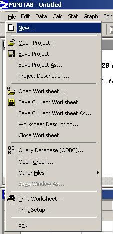
On the main menu bar, click on
"File".
Then click on "New...".
On the main menu bar, click on
"File". |
|
|
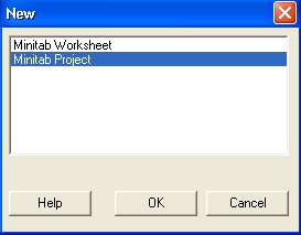
Click on "Minitab Project" and A new project will open, with no data in the single worksheet. |
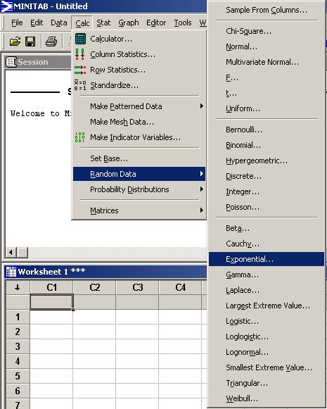
A particular type of lamp filament is known to have a life time that is a random quantity with an exponential distribution. The true mean lifetime of the filaments is known to be 1,000 hours.
Simulate a random sample of 100 such lamp filaments by placing
100 values, drawn randomly from an exponential distribution of
mean
On the main menu bar, click on "Calc". Then place the cursor over "Random Data". Then click on "Exponential...". |
|
Click in the box next to
"Generate".
Type 100
Click in the box under "Store in column(s):"
(or just press the Tab key).
Type C1
Click in the box next to "Scale:"
(or just press the Tab key).
Type 1000.
Leave the "Threshold:" box at its default value of zero.
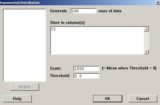
Click the "OK" button.
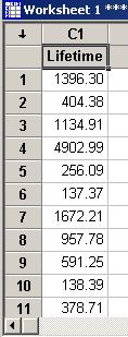
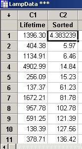
Give column [Note that your values will not be identical to the values that you see here. Every new generation of random values from a probability distribution will yield a new set of values.] As the sorted version of these data will appear in column
|
|
(Don’t forget to save your work often!)
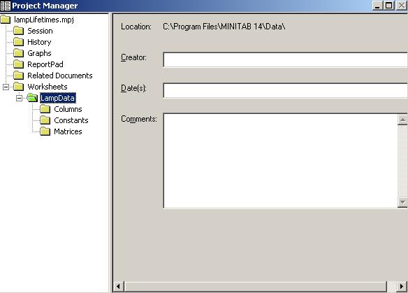
A data sheet can be renamed from the default "Worksheet 1" to a more meaningful name in Minitab’s Project Manager.
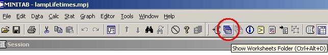
One way to access the appropriate part of the Project Manager is to click on the "Show Worksheets Folder" icon.
Another way is to summon the Project Manager to the top of the stack of Windows through the "Window" menu (or through the equivalent keystroke
|
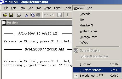
|
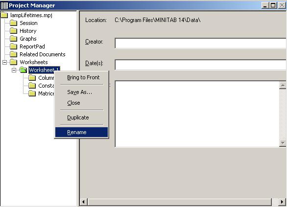
In the left pane of the Project
Manager, right-click on "Worksheet 1".
In the resulting pop-up menu, click on "Rename".
Type the new name for the worksheet
and press Enter.
|
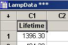
The data sheet has now been renamed. |
Although this step is not required by the problem specification, let us sort the data into ascending order.
In the Data window (not shown here), give an
appropriate name, such as "Sorted",
to column C2.
|
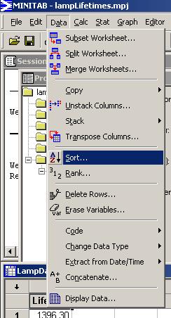
On the main menu bar, click on "Data". Then click on "Sort...". |
In the left pane, double-click
on the variable name for column C1.
It appears in the top right box, under "Sort column(s):".
Press the Tab key (or use the mouse), to place
the cursor in the next box, beside the first
"By column:".
In the left pane, double-click on the variable name for column
C1.
It appears in the first "By column:" box.
Click on the lowest radio button, "Column(s) of current
worksheet:".
Click in the text box below.
In the left pane, double-click on the variable name for column
C2.
It appears in the "Column(s) of current worksheet:"
box.
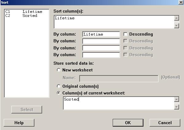
Click on the "OK" button.
|
The sorted version of your data should now be in the second column of your Data window. [Again, your values won’t match the values that you see here!] Note that values in the cells of the Data window are rounded
to two decimal places. In Minitab 14 the active cell,
(row 1
column |
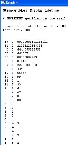
The first stem-and-leaf diagram needs between seven and twelve
stems.
The data range lies inside (0, 5500).
[Your range may be very different.]
Thus an interval of 500 is ideal and the leaf unit will be 100.
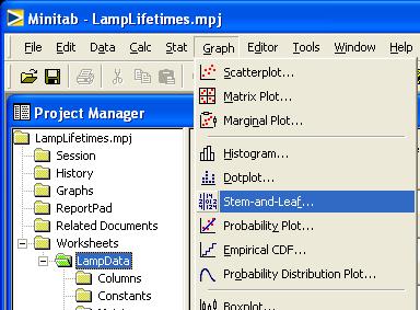
On the main menu bar, click on "Graph". Then click on "Stem-and-Leaf...". |
|
|
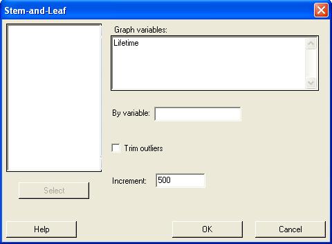
In this dialog box, Double click on the variable "Lifetime" Click in the box beside "Increment:" Click on the "OK" button. |
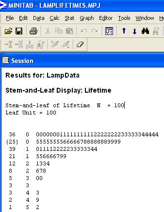
The results appear in the session window. 36 values lie in [0, 500). ... and so on, up to ... 1 value lies in [5000, 5500). |
|
|
Repeating the process, We can see that the median falls between two classes: 50 observations are at or below the 700’s and the other 50 observations are at or above the 800’s. Your stem and leaf diagram may look very different. Minitab 15 retains an inappropriate leaf of 100, while Minitab 13 resets the leaf unit to 10 (so that stems beyond 1000 are double-digits). |
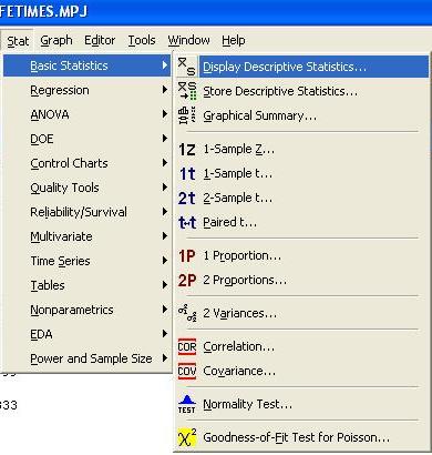
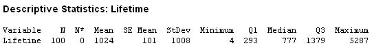
On the main menu bar, click on "Stat". Then place the cursor over "Basic Statistics". Then click on "Display Descriptive Statistics...". |
|
|
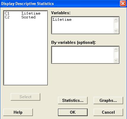
In the left pane, double click on either variable name. It appears in the top right box. [If you wish to change which items are displayed in the summary statistics, then click on the "Statistics..." button, check the boxes for the desired items and uncheck the other boxes.] Then click on the "Graphs..." button. |
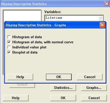
Check the boxes beside Then click on the "OK" button for this window. Click on the other "OK" button. |
|
These statistics appear in the Session window.
Two other windows have appeared.
The default boxplot shows four outliers (all more than one and a half
interquartile ranges above the upper quartile and some of them more than
three interquartile ranges above the upper quartile) and a pronounced
positive skew:
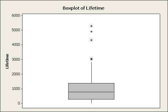
Again, by double-clicking on the graph, one can modify various features (not demonstrated here).
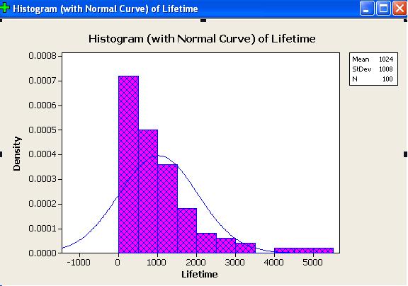
The default histogram incorporates many of our other results:
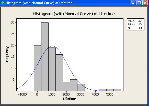
The random sample illustrated here came from an exponentially distributed population with a true mean of 1,000 hours. Yet the sample mean is just over 1023 hours. A good batch, perhaps, but not that unlikely to have occurred by chance, (as we shall be able to prove, after we have studied continuous probability distributions).
The distribution of the sample is clearly inconsistent with a normal distribution (the blue bell shaped curve). This is no surprise, as the true exponential distribution is strongly non-normal.
The positive skew is so strong that, although the sample
mean lamp filament lifetime is about 1023 hours, half of all
of the lamp filaments in this sample burned out in less
than 777 hours!
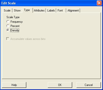
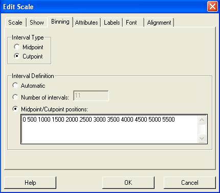
We require a true histogram (where the area, not the height, of each bar represents the frequency in that interval), with seven to twelve equal-width bars spanning most of the range (0, 5500).
Bar widths of 500, starting at 0, are ideal.
Rather than starting from scratch, let us modify the
default histogram.
Double click on any number by the vertical axis.
On the "Edit Scale" dialog box: Click on the third tab "Type"; Click the third radio button "Density"; and click the "OK" button. |
|
Back on the histogram, double click on any number by the horizontal axis.
|
On the "Edit Scale" dialog box: Click on the third tab "Binning". In the upper group, In the lower group, In the text box, enter values, Click the "OK" button. |
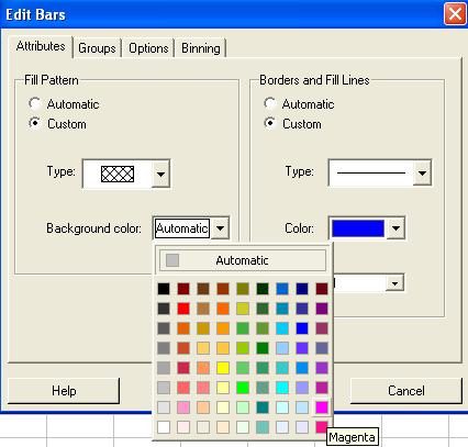
If you wish, you may also modify the visual appearance of the bars. Double-click inside any bar. On the first tab "Attributes" of the "Edit Bars" dialog box, click the respective "Custom" radio buttons |
|
Here is one version of the modified histogram:
You can copy and paste the above results into your Report Pad.
Then save your work and exit.