ENGI 3423 Probability and Statistics

Faculty of Engineering and Applied Science
2010 Fall

Solutions to Some Practice Questions for Test 2

The probability mass function for X = the number of major defects in a randomly selected appliance of a certain type is

x 0 1 2 3 4

p(x) .08 .15 .45 .27 .05

Compute
1. E [ X ]
2. V [ X ] directly from the definition
3. the standard deviation of X.
4. V [ X ] using the shortcut formula
These answers can be found by entering the values of the probability mass function into the Excel file demos/Discrete.xls, (which has been done in the associated Excel file).

x	0	1	2	3	4
p(x)	.08	.15	.45	.27	.05

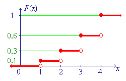
The discrete random quantity X has the following probability mass function:

x 1 2 3 4

p(x) .1 .2 .3 .4
1. Verify that p(x) is a valid p.m.f.
  - All four non-zero probability masses are positive.
  - å p(x) = .1 + .2 + .3 + .4 = 1
  Therefore p(x) is a valid p.m.f.
2. Sketch the cumulative distribution function F (x).
  
  The graph has the classic staircase appearance of the c.d.f. of any discrete random variable. The height of the gap between any consecutive pair of steps is equal to the probability mass at that step up. The graph then follows immediately.
3. Find the population mean of X.
  
  µ = E[X] = å x . p(x) = (1 × .1) + (2 × .2) + (3 × .3) + (4 × .4)
  = .1 + .4 + .9 + 1.6 = 3.0
  
  Another way to perceive this population mean is that an ideal ruler with point masses of .1, .2, .3 and .4 grammes at x = 1, 2, 3, 4 respectively, will balance at x = 3.
4. Find the population variance of X.
  
  Either
  
  s² = V[X] = å (x - µ)² . p(x) =
  ((1 - 3)² × .1) + ((2 - 3)² × .2) + ((3 - 3)² × .3) + ((4 - 3)² × .4)
  = .4 + .2 + 0 + .4 = 1.0
  
  or
  
  E[X²] = å x² . p(x) = (1² × .1) + (2² × .2) + (3² × .3) + (4² × .4)
  = .1 + .8 + 2.7 + 6.4 = 10.0
  
  Þ s² = V[X] = E[X²] - (E[X])² = 10.0 - (3.0)²
  = 10 - 9 = 1
5. Find the probability that the sample mean is less than 2.9 .
  
  The sample size is sufficiently large for the distribution of the sample mean to be normal to an excellent approximation, with mean µ and variance s² / n .
  Thus
  ~ N(3, (1 / 100) ) = N(3, 0.01).
  Þ P[ < 2.9] = P[Z < (2.9 - 3.0) / 0.1]
  = F(-0.1 / 0.1) = F(-1.00) = .1587
6. Find the probability that the sample mean is less than 2.0 .
  
  P[ < 2.0] = P[Z < (2.0 - 3.0) / 0.1]
  = F(-1 / 0.1) = F(-10) << 0.0001 (extremely unlikely; almost impossible)
  Thus
  P[ < 2.0] » 0

x	1	2	3	4
p(x)	.1	.2	.3	.4

A small town situated on a main highway has two gas stations, A and B. Station A sells regular, extra, and premium gas for 109.9, 111.1, and 114.4 cents per litre, respectively, while B sells no extra, but sells regular and premium for 108.9 and 114.4 cents per litre, repectively. Of the cars that stop at station A, 50% buy regular, 20% buy extra, and 30% buy premium. Of the cars stopping at B, 60% buy regular and 40% buy premium. Suppose that A gets 60% of the cars that stop for gas in this town, while 40% go to B. Let R = the price per litre paid by the next car that stops for gas in this town.
1. Compute the p.m.f. of R. Then draw a probability bar chart of the p.m.f.
  
  A tree diagram may be the easiest way to establish the p.m.f.
  
  the p.m.f. of R is
  
  P[R = 108.9] = P[(Station B) (regular)] = P[(Station B)] × P[ (regular) | (Station B)]
  = .4 × .6 = .24
  
  P[R = 109.9] = P[(Station A) (regular)] = P[(Station A)] × P[ (regular) | (Station A)]
  = .6 × .5 = .30
  
  P[R = 111.1] = P[(Station A) (extra)] = P[(Station A)] × P[ (extra) | (Station A)]
  = .6 × .2 = .12
  
  P[R = 114.4] = P[{(Station A) (premium)} {(Station B) (premium)}]
  = P[(Station A)] × P[(premium) | (Station A)]
  + P[(Station B)] × P[(premium) | (Station B)]
  = (.6 × .3) + (.4 × .4) = .34
  
  The bar chart should have four equal-width bars, centred on r = 108.9, 109.9, 111.1 and 114.4, with heights .24, .30, .12 and .34 respectively.
2. Compute and graph the c.d.f. of R.
  
  The c.d.f. is a classic staircase function.
  The height of each step is the value of the p.m.f. at that step.
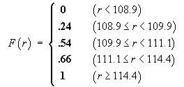
  The c.d.f. is
3. If a randomly chosen customer has purchased regular gas, then what is the probability that the gas was purchased at station A?
  
  P[(station A) | (regular)] = P[(station A) (regular)] / P[(regular)]
  From the tree diagram, P[(regular)] = .30 + .24 = .54.
  Therefore P[(station A) | (regular)] = .30 / .54 = 5 / 9 = .5555...

A box of silicon wafers will be withdrawn from a production line for more intensive testing, if and only if more than one defective wafer is found in a random sample of 20 wafers, drawn with replacement from the box.
Let p be the true proportion of defective wafers in the box.
Let X be the number of defective wafers in the random sample.
1. Show that the probability distribution for X is exactly binomial.
  - Each trial [wafer] consists of a pair of complementary outcomes, (defective or good).
  - P[defective] = constant (= p).
  - Trials are independent (the sample is drawn with replacement).
  - The sample size is constant (n = 20).
  All four conditions are satisfied exactly.
  Therefore the exact probability distribution is binomial, P[X = x] = b(x; 20, p).
2. Find, in terms of p, the probability that the box will be withdrawn from the production line for more intensive testing.
  
  P[box withdrawn] = P[X > 1] = 1 – P[X < 1] = 1 – B(1; 20, p)
  = 1 – (b(0; 20, p) + b(1; 20, p)) = 1 – ((1 – p)²⁰ + 20 p(1 – p)¹⁹) =
  
  1 – (1 + 19p)(1 – p)¹⁹
3. Evaluate the probability in part (b) in the case when p = .05 .
  
  When p = .05,
  1 – (1 + 19p)(1 – p)¹⁹ = 1 – (1 + 19×.05)(.95)¹⁹
  
  P[box withdrawn] = .2642 (4 d.p.)

The joint probability mass function p(x, y) for a pair of discrete random quantities X, Y is defined by the following table.

p		y
		–1	0	1
x	–1	.10	.05	.10
	0	.15	.20	.15
	1	.10	.05	.10

Find the correlation coefficient r for X and Y .

Extend the table to find the marginal p.m.f.s:

p_Y (y)		.35	.30	.35	1
p		y			p_X (x)
		–1	0	1
x	–1	.10	.05	.10	.25
	0	.15	.20	.15	.50
	1	.10	.05	.10	.25

E[X] = 3 x p_X (x) = –1×.25 + 0×.50 + 1×.25
= –.25 + 0 + .25 = 0
OR
X is symmetric about x = 0 implies

E[X] = 0

E[Y] = 3 y p_Y (y) = –1×.35 + 0×.30 + 1×.35
= –.35 + 0 + .35 = 0
OR
Y is symmetric about y = 0 implies

E[Y] = 0

E[XY] = 3 xy p (x, y) = –1×–1×.10 + 0 + –1×1×.10

+ 0 + 0 + 0

+ 1×–1×.10 + 0 + 1×1×.10

= 0

Cov[X, Y] = E[XY] – E[X]E[Y] = 0

s_X and s_Y are obviously positive, (X, Y are not absolute constants)
implies

r = 0.

Are X and Y stochastically independent?
Independence requires p (x, y) = p_X (x) p_Y (y) for all (x, y)
But p_X (–1) × p_Y (–1) = .35 × .25 = .0875 , while p (–1, –1) = .1000
Therefore p (–1, –1) ¹ p_X (–1) × p_Y (–1)
Therefore

NO, X, Y are not independent.

[This demonstrates that zero correlation does not guarantee independence,
(although the converse is true: independence does guarantee zero correlation).]
Also see the associated Excel file.

The probability density of a random quantity X is given by:
1. Find the value of k
  There are two conditions for f (x) to be a p.d.f.
  - f (x) > 0 for all x:
    This condition is true (trivially) outside the interval 0 < x < 2 .
    In the interval 0 < x < 2 we have (4 – x²) > 0 and x > 0.
    Therefore k > 0.
  - The coherence condition:
    It saves time to find the c.d.f. first, in terms of k, (done in part (b) below), then to set that function equal to 1 at the highest possible value of x.
    From part (b) below, F(x) = k x² (8 – x²) / 4 for 0 < x < 2
    But F(2) = 1 k (8 – 4) = 1
    k = 1/4
  The two conditions together require
  
  k = 1/4
2. Find the corresponding cumulative distribution function F (x)
  The c.d.f. is obviously F (x) = 0 for all x < 0 and is F (x) = 1 for all x > 2.
  Inside the interval 0 < x < 2 the c.d.f. is
  $F(x) = 0 + Integral_0^x {kt(4-t^2)} dt$
  $= k Integral_0^x {(4t-t^3)} dt = k [2t^2 - t^4/4]_0^x$
  
  But, from part (a) above, k = 1/4
  Therefore
  $F(x) = {0, x^2 / 16 * (8-x^2), 1}$
3. What are the odds that a random quantity having this distribution will take on a value greater than 1?
  P[X > 1] = 1 – F (1) = 1 – (8 – 1) / 16 = 9/16
  
  Therefore the odds of P[X > 1] are
  
  9:7 on

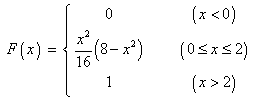
Suppose that the duration (in years) of a construction job can be modelled as a continuous random quantity t whose cumulative distribution function (c.d.f.) is given by
1. Find the probability that the construction job lasts longer than half a year.
  P[T > 0.5] = 1 – P[T < 0.5] = 1 – F (0.5) = 1 – (1 – 1/4)
  Therefore
  
  P[T > 0.5] = 1/4
2. Find the median duration , correct to two decimal places.
  The definition of the median is
  
  Clearly, from the definition of F (t) , the median must lie in the interval [0, 1].
  Solve 2 t – t² = 1/2
  t² – 2 t + 1/2 = 0
  
  Therefore
3. Determine the corresponding probability density function f (t).
  Where F (t) is constant, F' (t) = f (t) = 0.
  This is true outside the interval 0 < t < 1.
  
  Inside the interval 0 < t < 1 ,
  F (t) = 2 t – t²
  f (t) = 2 – 2 t
  
  f (t) = 2 (1 – t) (0 < t < 1)

Space craft are to be landed at some given point "O" on the moon�s surface, and we wish to observe the position of an actual landing point relative to the aiming point O. Assume that the landing errors are small enough so that it is reasonable to measure them in the tangent plane to the moon�s surface which touches O. Let us further establish a local rectangular coordinate system in that tangent plane which is centered on O and which is oriented so that the x axis points east and the y axis points north.

Suppose that the probability that the space craft lands more than 10 km from the aiming point O is zero and, further, that the probability that the spacecraft lands in some particular region (no point of which is more than 10 km from O) is directly proportional to the area of that region.

Find the probability that the space craft will land
1. less than 5 km from O
  
  The available landing area is the area contained by a circle, radius 10 km, centre at O, area = p×10² = 100p.
  Because the probability of landing in any region within the circle is proportional to the area A of that region, that probability must be A/(100p).
  
  Therefore P[lands < 5 km from O] = (Area of circle, radius 5) / (100p)
  = (25p) / (100p)
  
  = 1/4 = .25
2. more than 1 km yet less than 3 km from O
  Let X be the landing distance from O.
  P[1 < X < 3] = ((Area of circle, radius 3) – (Area of circle, radius 1)) / (100p)
  = (9p - p) / (100p)
  
  = 2/25 = .08
3. north of the aiming point
  
  Assuming that “north of the aiming point” means “anywhere in y > 0”, then the event covers exactly half of the sample space.
  Therefore
  
  P[lands north of the aiming point] = 1/2 = .5
  
  [If one assumes that “north of the aiming point” means “anywhere in the direction between north-west and north-east”, then the area is exactly one quarter of the sample space and the answer becomes 1/4.]
4. north-east of the aiming point
  
  Assuming that “north-east of the aiming point” means “anywhere in the first quadrant”, then the event covers exactly one quarter of the sample space.
  Therefore
  
  P[lands north-east of the aiming point] = 1/4 = .25
5. south of the aiming point and more than 5 km from O
  
  Assuming that “south of the aiming point” means “anywhere in y < 0”, then the event covers exactly half of the event “more than 5 km from O”.
  
  Therefore P[lands south of the aiming point and more than 5 km from O]
  = (1/2) × ((Area of circle, radius 10) – (Area of circle, radius 5)) / (100p)
  = (100 – 25) / (2 × 100)
  
  = 3/8 = .375
  
  [If one assumes that “south of the aiming point” means “anywhere in the direction between south-west and south-east”, then the area is reduced by a factor of two and the answer becomes 3/16.]
6. exactly due south of O.
  
  “Exactly due south of O” means anywhere on the negative y axis. This is a degenerate rectangle of height 10 km and width zero, giving zero area.
  Therefore
  
  P[lands exactly due south of O] = 0

Let X have the Pareto probability density function
$f(x; k, t) = { k*t^k /(x^(k+1)), x >= t ; = 0 , x < t$ where k and t are both positive parameters.
1. Find necessary conditions on k to ensure that E[Xⁿ] is finite.
  (n = a positive integer).
  $E[X^n] = Integral_t^infty{x^n * k*t^k / x^(k+1)}dx$
  
  Otherwise
  
  Therefore the necessary (and sufficient) condition on k for E[X ⁿ ] to be finite is
  
  k > n .
2. Hence find the range of values of k for which the variance V[X] is finite.
  
  V[X] = E[X ² ] – (E[X]) ²
  E[X ² ] is finite provided k > 2.
  E[X ] is finite provided k > 1.
  V[X] is finite iff E[X ² ] and E[X ] are both finite.
  
  Therefore V[X] is finite provided
  
  k > 2.
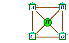
3. Find an expression (in a simplified form) for the variance when it is finite.

Adam Ant can travel only along the twigs connecting his home H with his aunts’ homes A, B, C, D, as shown in the diagram.
square grid; A, B, C, D at corners; H at centre
One fine day, Adam decides to visit his aunt at house A. Then it is time to return home. Being a confused young ant, his choice of route is random (equal probability for each twig). Let X = the number of aunts he visits before he next returns to his home. Thus X = 1 represents the event “Adam Ant returns to his home immediately after his initial visit to Aunt A” and P[X = 1] = 1/3 .

Find the probability mass function for the random quantity X.

At any of his aunts’ houses, one path leads home and the other two do not. Therefore
P[(Adam goes home immediately after visit x) | (Adam had not gone home before visit x)]
= P[X = x | X > x – 1 ] = 1/3
For the event (X = x) to happen, Adam must stay away from his home on all previous (x – 1) departures from aunts’ houses, (with a probability of 2/3 for each one). Therefore

Challenging questions:

Find E[X].
[Note: The sum s of a convergent geometric series with first term a and common ratio r is
s = a / (1 – r) .]

Therefore

E[X] = 3 .

OR

Note that the probability distribution is geometric, with parameter p = 1/3.
It then follows immediately that

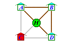
Show that the probability that Adam Ant never visits aunt C is 4/7.

There continue to be three equally likely paths from each of the aunts’ houses. However, we now wish to count only those paths that do not pass through house C.

For each value of x, each distinct path, (such as ABAH for x=3), has a probability of (1/3)^x.
House C removed from valid paths

We need to count the number n(x) of remaining valid paths for each value of x.
When x is odd, the final visit must be to aunt A or aunt D.
When x is even, the final visit must be to aunt B only.
It then follows that, when x is odd, n(x + 1) = n(x)
and when x is even, n(x + 1) = 2 n(x)
Also, n(1) = 1.
This recursive relationship allows us to build up the values of n(x):

x 1 2 3 4 5 6 7 8 9

n(x) 1 1 2 2 4 4 8 8 16

Thus n(x) = 2^{ceil(x/2) – 1}, where ceil(k) is k rounded up to the nearest integer.
The probability that Adam never visits house C then follows:

$prob. = Sum{ n(x) (1/3)^x }$
[separate into odd and even series]
[factor out common terms from both series]

[manipulate to obtain a geometric series,
sum S = 9/7]

[The odds are therefore 4 to 3 on that Adam never visits aunt C.]

OR [method based on a suggestion from Dr. Theodore Norvell]

Consider just the first one or two moves:

Path Probability Visit Aunt C ?

AH 1/3 NO

ABH 1/9 NO

ABA[...any...] 1/9 ?

ABD[...any...] 1/9 ?

AC[...any...] 1/3 YES

Thus (1/3 + 1/9 =) 4/9 of the time, Adam definitely does not visit aunt C.
(1/3 =) 3/9 of the time, Adam definitely does visit aunt C.
The remaining 2/9 of the time, the situation remains unresolved after two moves, with Adam visiting either aunt A again or aunt D.

Path	Probability	Visit Aunt C ?
AH	1/3	NO
ABH	1/9	NO
ABA[...any...]	1/9	?
ABD[...any...]	1/9	?
AC[...any...]	1/3	YES

Let p represent the probability that Adam never visits aunt C before he returns home.
Whenever Adam is setting out from the house of aunt A,
P[Adam never visits C | Adam is at A] = p
(because the situation is exactly the same as it was the first time that he set out from aunt A)
and, by symmetry,
P[Adam never visits C | Adam is at D] = p
Bringing all the [mutually exclusive] cases where Adam does not visit aunt C together,
p = P[AH] + P[ABH] + P[Adam never visits C and (ABA or ABD)]
= (P[AH] + P[ABH]) + (P[ABA or ABD] × P[Adam never visits C | (ABA or ABD)])

as before.

What are the odds that Adam Ant visits both aunt B and aunt C at least once?

Let B = “Adam visits aunt B at least once”
and C = “Adam visits aunt C at least once”,
then, by symmetry, P[B] = P[C] (= 1 – 4/7 = 3/7).

However, events B and C are neither independent nor incompatible.
The only way in which Adam can avoid visiting both aunts B and C is by proceeding home directly from the initial visit to aunt A, the probability for which is P[X = 1] = (1/3).

Therefore the required odds are

17:4 against

A certain atmospheric sensing device has an advertised service life of one year, but it is vulnerable to severe icing. If it survives the full year, then the profit to the owner is 50 (in some units of currency). If an ice storm severe enough to be fatal to the device occurs during its service life, then the profit is reduced by 90 units, unless the owner had invested in protection (costing 15 units), in which case the profit is reduced by 20 units.

An analysis method is available (at a cost of 5 units) which will suggest whether or not such icing will occur during the service life of the device. The analysis is not perfect: in only 95% of all cases where icing fatal to the device occurs, the analysis correctly suggests that such icing will occur. The analysis also suggests fatal icing (incorrectly) in 20% of all cases when no such icing happens.

It is also known from past experience that the probability of icing fatal to the device during the year is 20%.

Given that the analysis suggests that fatal icing will occur, find the probability that such icing happens.

Let I = fatal icing occurs during the year
and A = analysis suggests I will occur.
Then, from the question,
P[I] = .20,
P[A | I] = .95 implies P[~A | I] = .05 and
P[A | ~I] = .20 implies P[~A | ~I] = .80 .

P[I | A] is wanted. Use Bayes’ theorem.

Tree diagram version of Bayes’ theorem:

Total probability law:
P[A] = P[AI] + P[A~I] = .19 + .16 = .35
Complementary event:
P[~A] = 1 – .35 = .65
Conditional probability:
P[I | A] = P[I A] / P[A] = .19 / .35
[Bayes' calculation tree]

= 19/35 = .5429 (to 4 d.p.)

Given that the analysis suggests that fatal icing will not occur, find the probability that such icing does happen.
Conditional probability (from part (a)):
P[I | ~A] = P[I ~A] / P[~A] = .01 / .65

= 1/65 = .0154 (to 4 d.p.)

Construct a decision tree for this problem and determine the optimum strategy for the owner.

The complete tree diagram is available on an Excel spreadsheet.
Some calculations are described below:
[Decision tree]

Folding back:
a = (19/35)×10 + (16/35)×30 = 134/7
b = (19/35)×(–45) + (16/35)×45 = –27/7
a > b
Therefore choose a and
g = a = 134/7

c = (1/65)×10 + (64/65)×30 = 386/13
d = (1/65)×(–45) + (64/65)×45 = 567/13
d > c
Therefore choose d and
h = d = 567/13

e = (1/5)×15 + (4/5)×35 = 31
f = (1/5)×(–40) + (4/5)×50 = 32
f > e
Therefore choose f and
j = f = 32

Folding back to the left-most node,
k = (35/100)×(134/7) + (65/100)×(567/13) = 701/20 = 35.05
j = 32.00
k > j
Therefore choose k and
Expected profit = k = 701/20

The optimum strategy is therefore

Pay 5 for the analysis
If the analysis suggests icing, then invest in protection.
Otherwise don’t invest in protection.

The expected profit is 35.05 units.
The actual profit is one of:
–45 (occurs 1% of the time), +10 (19% of the time),
+30 (16% of the time) or +45 (64% of the time).

A box contains 12 good items and 3 defective items from a factory’s production line. A manager selects four items at random from the box, without replacement.
Let X = (the number of defective items in the random sample).
1. Show that the probability distribution of X is not binomial.
  
  Test the four conditions for a binomial distribution:
  - Each trial has a complementary pair of outcomes (good/defective) True.
  - P[success] is constant (= 3/15). True.
  - Trials are independent. False.
    P[item 2 defective | item 1 defective] = 2 / 14 P[item 2 defective]
  - Number of trials constant (= 4) True.
  The failure of the independence condition occurs because the sampling is without replacement.
2. Find the probability mass function p(x).
  
  x must lie between 0 and 3 (the number of successes in the sample cannot exceed the total number of successes in the entire population). Thus p(x) must be zero except at x = 0, 1, 2 and 3.
  
  n(S) = (the number of ways of drawing 4 items from 15 without restriction) = ¹⁵C₄.
  n(E) = (the number of ways of drawing x successes from the 3 successes in the population and (4 – x) failures from the 12 failures in the population) = ³C_x × ¹²C_{4 – x}.
  
  Therefore the p.m.f. is
  
  p(x) = ³C_x × ¹²C_{4 – x} / ¹⁵C₄ , (x = 0, 1, 2, 3 only).
  
  [The numerical values are p(x) = .3626, .4835, .1451 and .0088 for x = 0, 1, 2 and 3 respectively.]
  
  [This is a hypergeometric probability distribution.]
3. Find P[X = 4] (Note: this part can be attempted without part (b)).
  
  As noted above, it is impossible to draw more defective items without replacement than are present in the population.
  Therefore P[X = 4] = 0.
4. Find P[X < 3] .
  
  P[X < 3] = 1 – P[X = 3]
  = 1 – ³C₃ × ¹²C_{4 – 3} / ¹⁵C₄ = 1 – 1 × 12 / 1365 = 1353 / 1365
  = .9912
5. If the random sample were drawn with replacement, would the probability mass function be binomial?
  
  YES:
  Sampling with replacement will make the third condition in part (a) above true.
6. If the random sample were drawn with replacement, what would the value of P[X = 4] be?
  
  P[X = 4] = b(4; 4, .2) = ⁴C₄ (.2)⁴ (.8)⁰
  = .0016

Also see the Term Tests from the years 2008, 2007 and 2006.

[Return to the index of assignment solutions.]

[Return to your previous page.]

Created 2004 09 02 and most recently modified 2010 07 30.

E[XY] = 3 xy p (x, y) =	–1×–1×.10 + 0 + –1×1×.10
	+ 0 + 0 + 0
	+ 1×–1×.10 + 0 + 1×1×.10
	= 0