ENGI 4421 - Second MINITAB Tutorial

In this session we shall use Minitab^® to
•   generate values from a probability distribution,
•   sort those values into ascending order,
•   generate summary statistics using Minitab’s defaults for these data,
•   create a custom histogram for these data.
•   open a new (blank) project,
•   create a macro file for use in Minitab,
•   execute the macro file in Minitab,
•   produce an empirical estimate of probability for the event
  “A fair coin lands heads up”.
•   produce an empirical estimate of probability for the event
  “At least two of n people in a room share the same birthday”.
Also provided on this web page are
•   A note about file extensions
•   Some Notes on Macro Syntax
•   Macro code:   detecting equal values in a column

Simulation Example #1 - Lamp Lifetimes

A particular type of lamp filament is known to have a life time that is a random quantity with an exponential distribution.   The true mean lifetime of the filaments is known to be 1,000 hours.

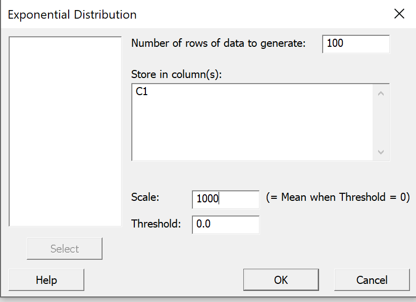
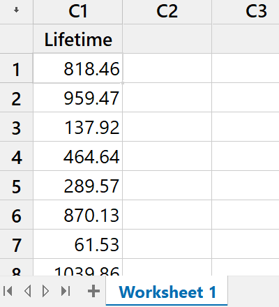
Simulate a random sample of 100 such lamp filaments by placing 100 values, drawn randomly from an exponential distribution of mean µ = 1000, in a column in a Minitab worksheet.   Generate the following descriptive statistics in Minitab for your sample:

•   a list of descriptive statistics (mean, median, etc.)
•   a graphical summary
•   a separate boxplot
•   an histogram with seven or eight equal-width classes
 

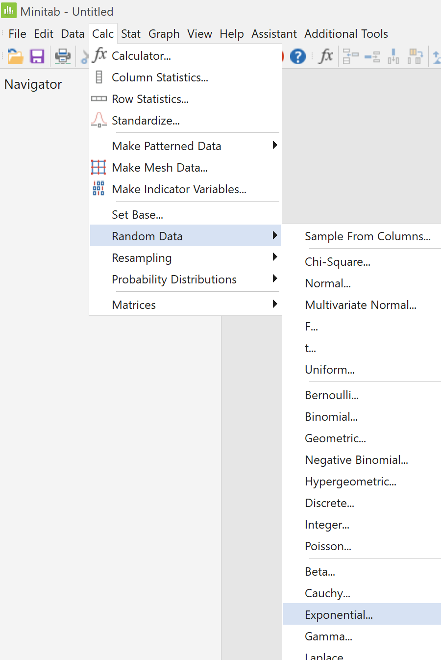
Generating Random Values

On the main menu bar, click on "Calc". Then place the cursor over "Random Data". Then click on "Exponential...".

---




Click in the text box next to "Number of rows to generate". Type 100 Click in the box under "Store in column(s):"   (or just press the Tab key). Type C1 Click in the box next to "Scale:" (or just press the Tab key). Type 1000. Leave the "Threshold:" box at its default value of zero. [The "Threshold:" parameter is the lowest possible value, which is also the mode for an exponential distribution.] Click the "OK" button.

---




Give column C1 a meaningful name. [Note that your values will not be identical to the values that you see here. Every new generation of random values from a probability distribution will yield a new set of values.]




(Don’t forget to save your work often!)

---

If you wish, you can save the data sheet separately from the entire Minitab project. Click anywhere on the data pane to ensure that it is the active pane. From the 'File' menu click on 'Save Worksheet As ...' then save the worksheet as a Minitab .mwx file in a location and with a name of your choice.

 

Sorting Data

---

Although this step is not required by the problem specification, let us sort the data into ascending order.

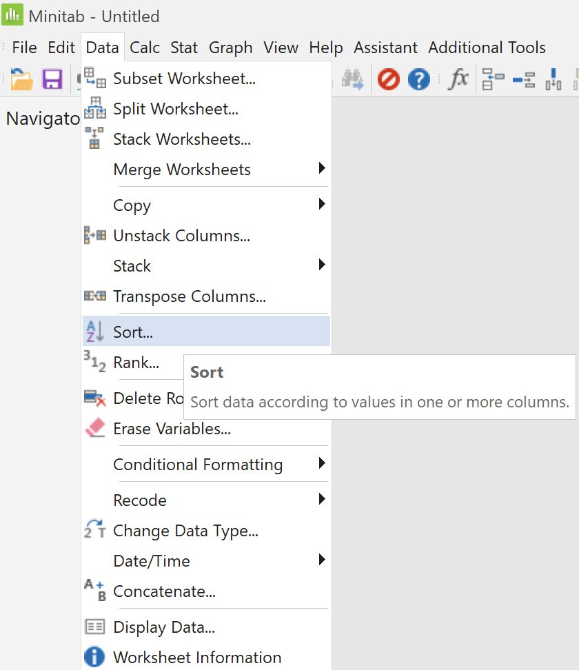
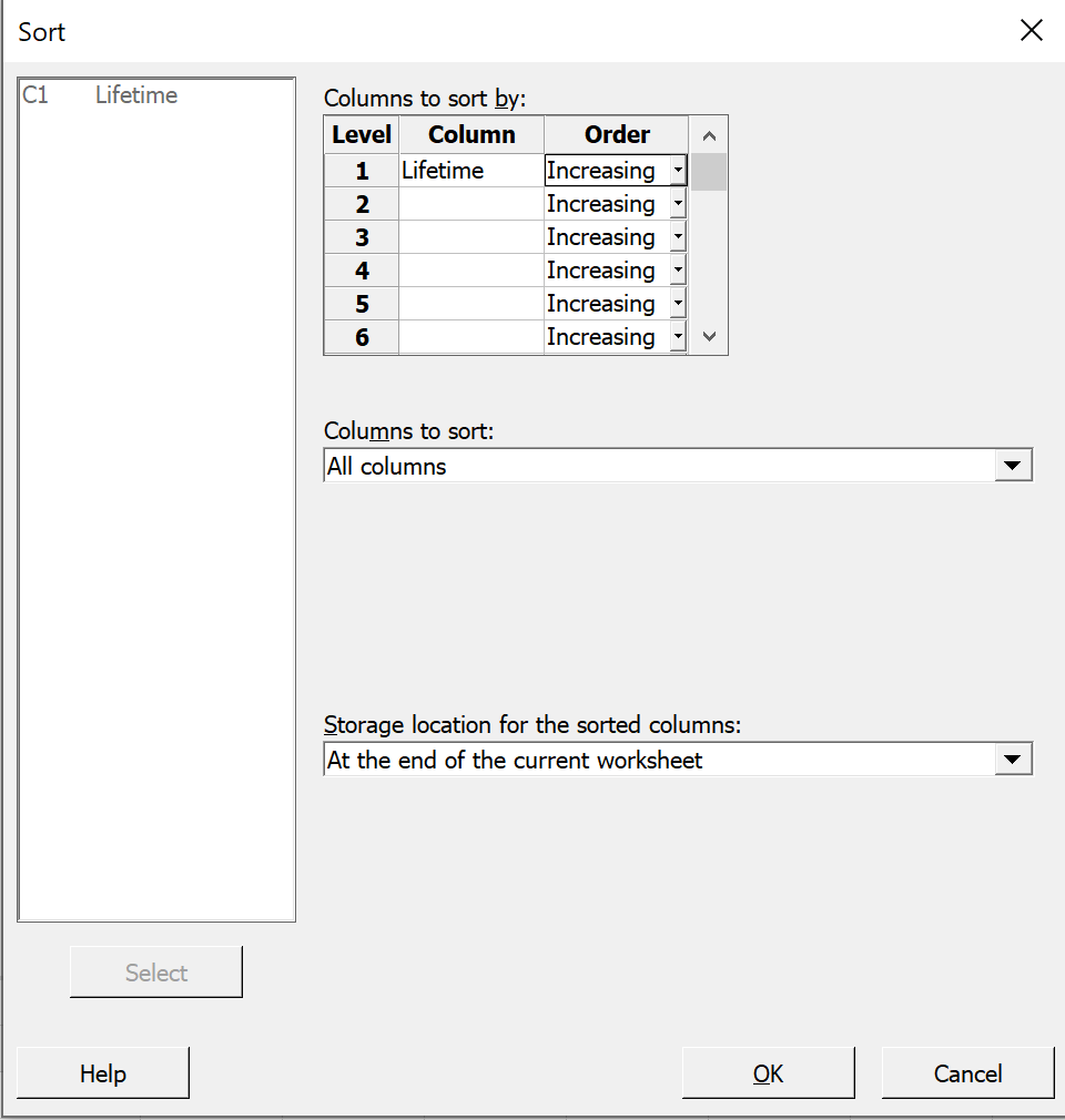
On the main menu bar, click on "Data". Then click on "Sort...".

---




In the left pane, double-click on the variable name for column "C1 Lifetime". It appears in the top right box, in the cell for "Column" and Level 1. Accept all the other defaults. The 'Sort' dialog box should now look like this.         Click on the "OK" button.

---

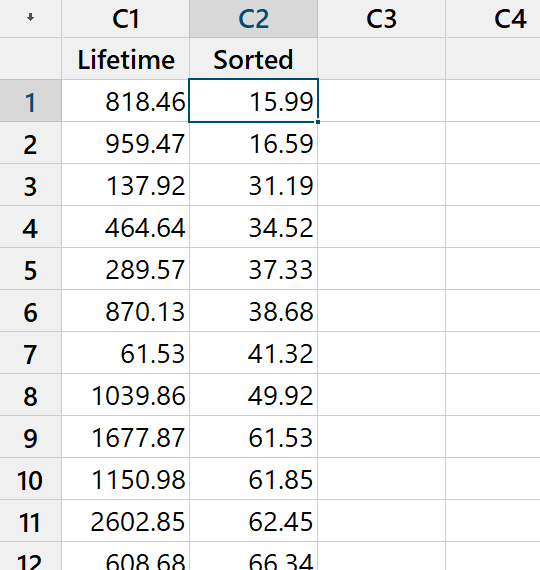
The sorted version of your data should now be in the second column of your worksheet. [Again, your values won’t match the values that you see here!] By clicking in the column header, one can amend the column's alias.   Here I have shortened 'Sorted Lifetime' to just 'Sorted'. Note that values in the cells of the worksheet in the data pane are rounded by default to two decimal places. Through a menu that pops up upon right-clicking on a cell, one can force Minitab to display more or fewer decimal places (not shown here).

 

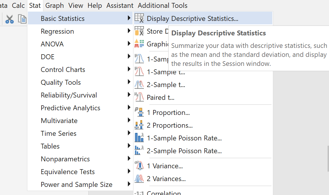
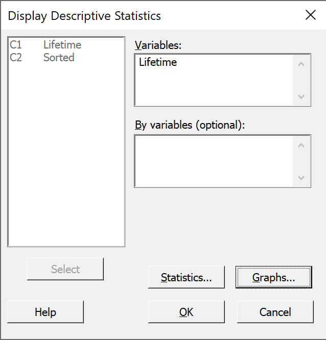
Descriptive Statistics

In tutorial #1 we saw how to obtain summary statistics.   Nevertheless, we shall repeat the process here. On the main menu bar, click on 'Stat'. Then place the cursor over 'Basic Statistics'. Then click on 'Display Descriptive Statistics...'.

---




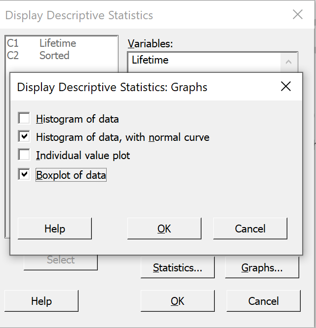
In the left pane, double click on either variable name. It appears in the top right box. [If you wish to change which items are displayed in the summary statistics, then click on the "Statistics..." button, check the boxes for the desired items and uncheck the other boxes, as we did in tutorial #1.] Then click on the "Graphs..." button.

---




Check the boxes beside 'Histogram of data, with normal curve' and 'Boxplot of data' Then click on the "OK" button for this window. Click on the other "OK" button.

---




These statistics appear in the output pane.



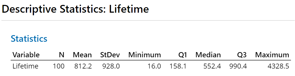
Again, your values will be different from these values.

---

Two plots have appeared in the output pane.
Scrolling down to the foot of the output pane, we find the default boxplot.

It shows several outliers (all more than one and a half interquartile ranges above the upper quartile and some of them more than three interquartile ranges above the upper quartile) and a pronounced positive skew:



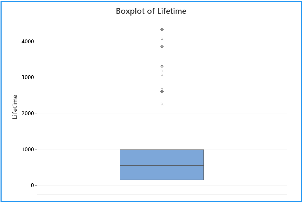
Again, by right-clicking on the graph and selecting 'Edit Graph...' on the pop-up menu, one can modify various features (not demonstrated here).

---

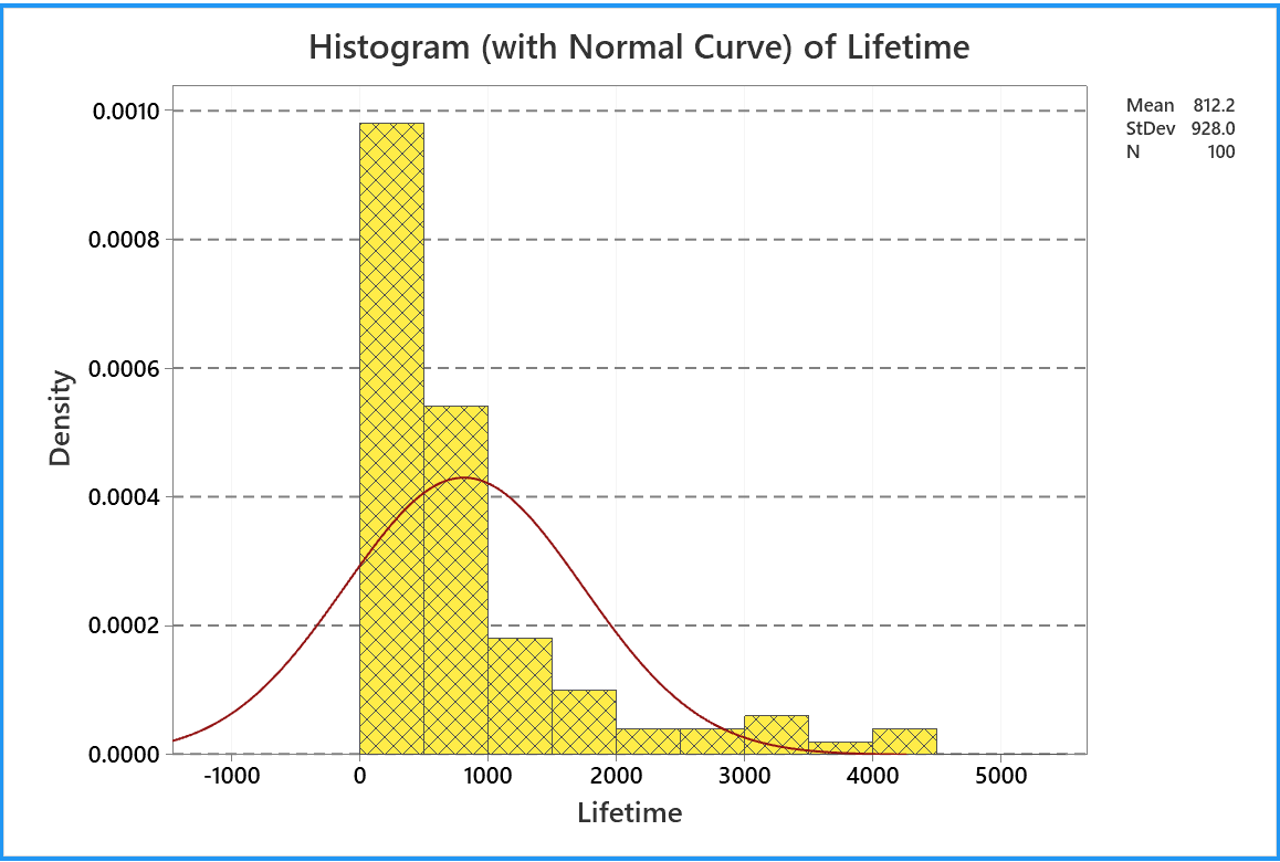
The default histogram incorporates many of our other results:



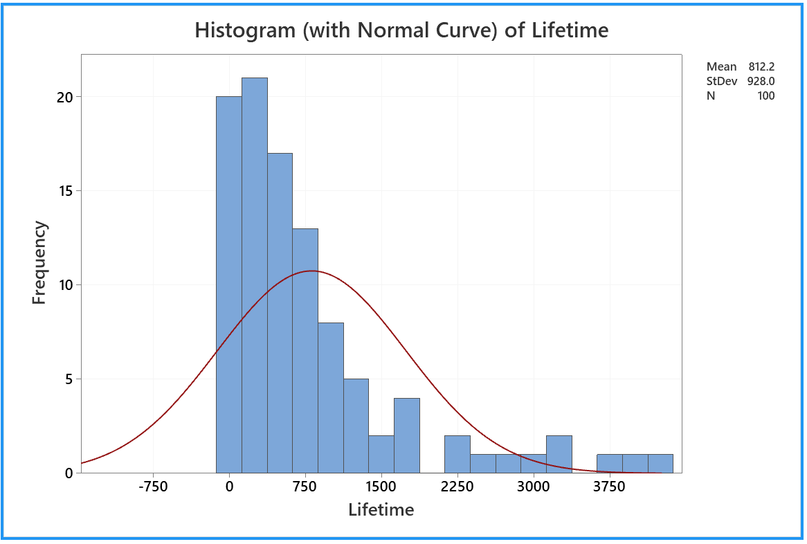
The random sample illustrated here came from an exponentially distributed population with a true mean of 1,000 hours.   Yet the sample mean is well under 900 hours.   A poor batch, perhaps, but not that unlikely to have occurred by chance, (as we shall be able to prove, after we have studied continuous probability distributions).

Sometimes, by chance, the sample mean and sample standard deviation are well over 1,000 hours. See if your simulation produces even more extreme outliers.

The distribution of the sample is clearly inconsistent with a normal distribution (the red bell shaped curve).   This is no surprise, as the true exponential distribution is strongly non-normal.

The positive skew is so strong that, although the sample mean lamp filament lifetime in this sample is just over 810 hours, half of all of the lamp filaments in this sample burned out in less than 560 hours!

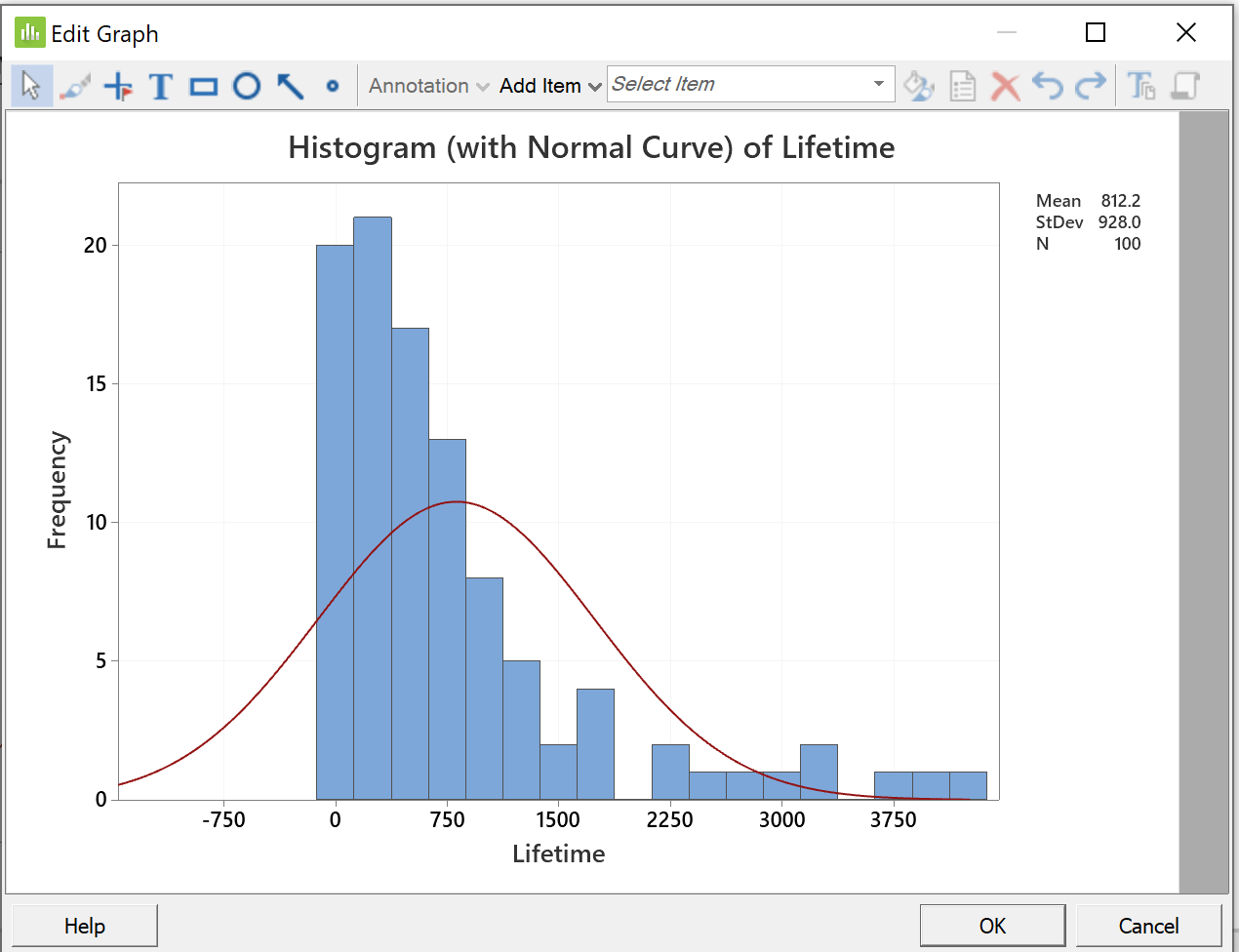
Custom Histogram

---

We require a true histogram (where the area, not the height, of each bar represents the frequency in that interval), with seven to twelve equal-width bars spanning most of the range (0, 5500).

Bar widths of 500, starting at 0, are ideal.

Note that the maximum value in my sample is under 4500 hr (which is quite low).   If your sample has a maximum value above 5500, then add further bars of width 500 as necessary.

Rather than starting from scratch, let us modify the default histogram.
Double click on any part of the default "histogram" to bring up the 'Edit Graph' window.



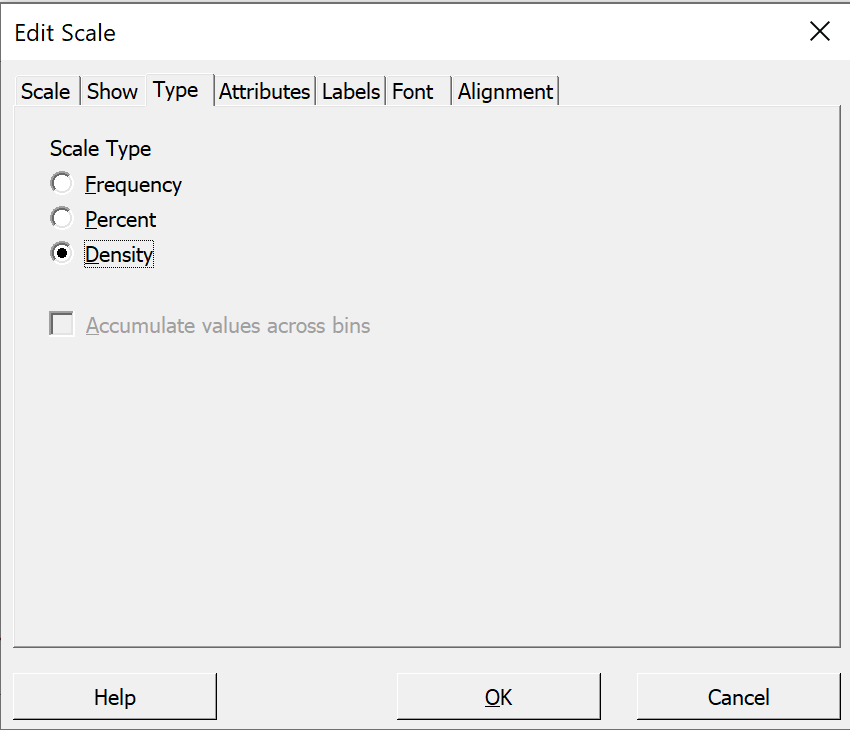
Double click on any number by the vertical axis.

---

On the "Edit Scale" dialog box: Click on the third tab "Type"; Click the third radio button "Density"; and click the "OK" button.

---




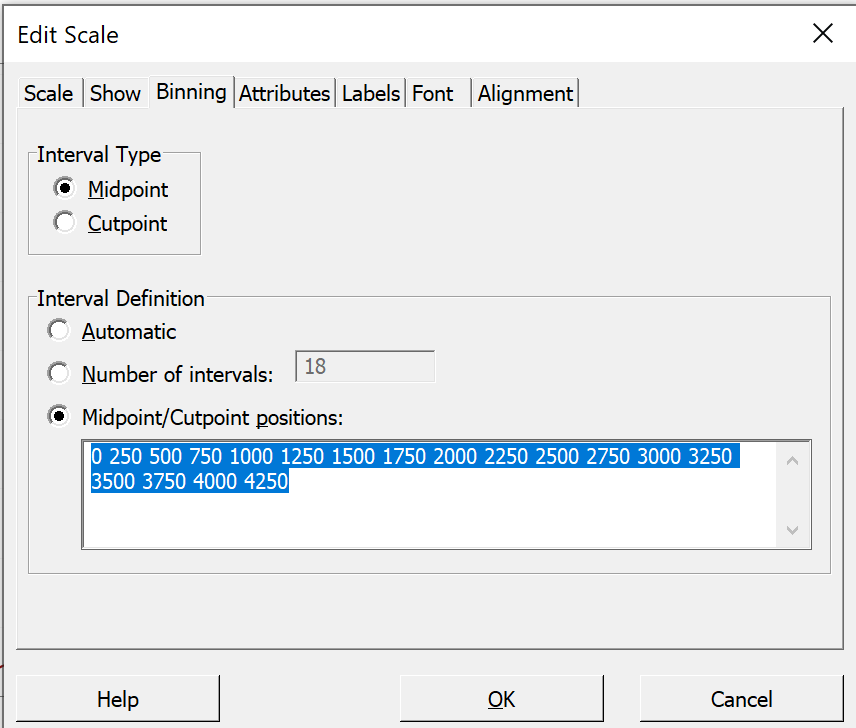
Back in the 'Edit Graph' window, double click on any number by the horizontal axis.

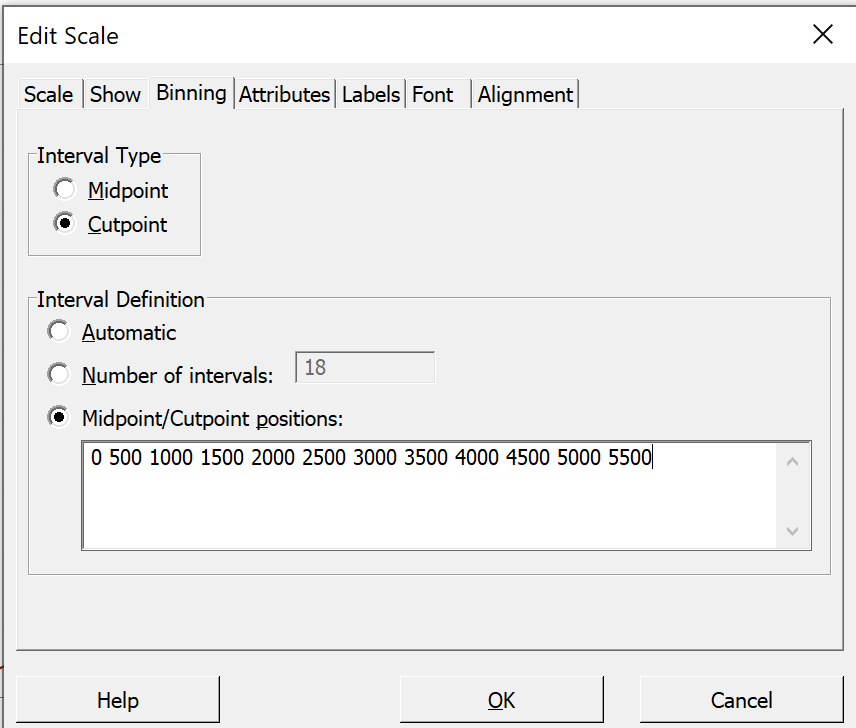
On the "Edit Scale" dialog box: Click on the third tab "Binning". In the lower group 'Interval Definition', Click the last radio button "Midpoint / Cutpoint positions:". In the text box, drag your cursor to select all values, then copy the selection into the clipboard (using any of 'Ctrl+Ins',   'Ctrl+C' or right-click on the selection and, in the pop-up menu, click on 'Copy').

---




In the upper group 'Interval Type', Click the second radio button "Cutpoint". The values of the bar boundaries in the text box vanish! Back in the lower group, click in the now-empty text box and paste the values back in. (This saves having to re-type all of the values). Now edit the values to run from 0 in multiples of 500 to the lowest multiple above your highest value. Click the "OK" button.

---




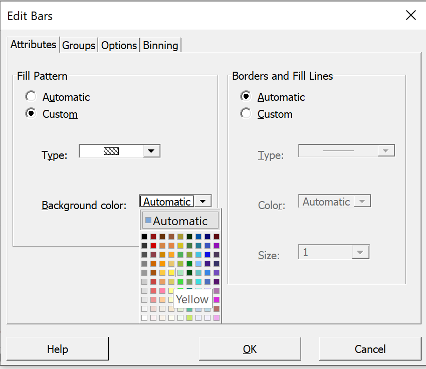
If you wish, you may also modify the visual appearance of the bars. Double-click inside any bar. On the first tab "Attributes" of the "Edit Bars" dialog box, click the respective "Custom" radio buttons and amend the bars as you see fit.

---




Here is one version of the modified histogram,
(with the horizontal gridlines made more visible, as in tutorial #1):



You can extract the above results into .rtf files.
Then save your work and exit.

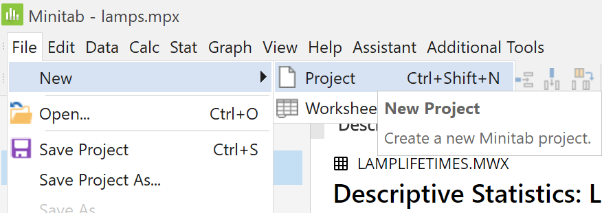
Open New Project

On the main menu bar, click on "File". Then hover on 'New >' and in the new pop-up menu, click on 'Project'. Minitab will give you a last chance to save the active project. A new project will then open, with no data in the single worksheet of the data pane and a blank output pane.

Simulation Example #2 - Coin Flips

Creation of a Macro File

Macros allow a repetitive set of Minitab commands to be executed all at once by invoking a macro file.   There are three main types of Minitab macros, but we will see only one of them (global) in this course.   More information is available at this Minitab link.

Copy the following block of text and paste it into a blank document in a word processor (even Notepad will suffice).
It is also available as a separate file at this link, (with a file name "Coins.txt" instead of "Coins.mac", because programs such as QuickTime insist on hijacking the '.mac' extension for image files instead of plain text Minitab macros).

---

gmacro
Coins
### Simulation to illustrate the evolution of the relative frequency of 
### heads as a fair coin is tossed many times.   The relative frequency 
### estimates the exact probability of 1/2 .
### Execute this macro in a blank Minitab project.
### Macro created 2003 03 14 and last modified 2021 02 16 by G.H. George

### mtitle / endmtitle needed to keep all output in one output pane
mtitle "Coin tossing simulation"
  erase c1-c3           # needed to ensure clear space in the worksheet
### Constants:
### k1 = coin index number (loop counter)
let k2 = 1500           # number of coins
let k3 = 0              # accumulator = number of heads in the first k1 coins

### Columns:
  name c1 'trial'       # number of coin tosses so far
  name c2 'head?'       # = 1 if this coin is a head, = 0 if a tail
  name c3 'Rel.Freq.'   # proportion of heads so far

### Place the first (k2) natural numbers into column c1:
  set c1
    1:k2
    end.
### assign 0 (tail), 1 (head) randomly to the k2 coins:
  random k2 c2;
    integer 0 1.
### toss the coin k2 times, recording number & proportion of heads so far:
  do k1=1:k2            
      let k3 = k3 + c2(k1)
      let c3(k1)=k3/k1
  enddo

  let k1 = c3(k2)
  note The last estimated probability of a head is
  print k1
  note Compare this with the true probability of 0.500000
### Plot the relative frequency as a time series plot: 
Tsplot 'Rel.Freq.';
  Scale 2;
    MODEL 1;
      Tick 0.3 0.4 0.5 0.6 0.7;
      Min 0.3;
      Max 0.7;
    EndMODEL;
  AxLabel 1;
    ADisplay 1;
    Label "# coins";
      ALevel 1;
  Index;
  Connect;
    Type 1;
    Size 2;
  Symbol;
    Type 0;
    Size 0.75;
  Title "ENGI 4421 Empirical Probability";
  SubTitle "Coin Tossing Experiment";
  Footnote;
    FPanel;
  NoDTitle.

endmtitle
endmacro

---

If you are using the computers in EN 3000/3029, then save the file on your Labnet account or on a USB stick, (using the file name "Coins.mac").

If you have a copy of Minitab on your own computer, then save the file in your Minitab Macros directory, (on some computers, it is at
"C:/Program Files/Minitab/Minitab 19/English/Macros/"), with the name "Coins.mac".

If there are any spaces in the file name or in any directory names in the path (except for the Minitab default on the C: drive noted above), then enclose the full file path/name in double quotes when invoking it.
Minitab does not like spaces in macro file names!
If the file is in a directory such as "My Documents" and double quotes are not used, then Minitab will not be able to find it.

---

A note about file extensions:

By default, Windows / Notepad insists on appending a hidden extension ".txt" to the name of your newly-created macro file (so that it is stored as "Coins.mac.txt" but displays in Windows Explorer, confusingly, as the desired "Coins.mac" .   However, Minitab recognizes only files whose names end with ".mac" to be macro files.   To escape from this problem, in Windows 10:

• open Windows Explorer
• at the top menu bar, click on 'View'
• check the box 'File name extensions'

.

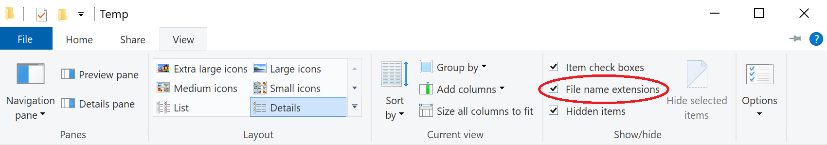Now inspect the name of your file.   If it ends in ".txt", then click on the file name and rename it to "Coins.mac".

The main alternative is to enclose the macro’s filename in double quotes in the "File name" field of the "Save As" dialog box, every time that you wish to save a macro file.

Some Notes on Macro Syntax

The first two lines of most Minitab global macros are


    gmacro
    macroName

and the last line is


    endmacro

The purpose of the mtitle / endmtitle command is to ensure that all output generated between the mtitle and the endmtitle appears in the same output pane, whose tab name is the string in double quotes following the mtitle.

The line indentation and blank lines are not required.
However, as is the case with any type of computer program, a macro is much easier to read if these style conventions are employed.

The comment symbol ("//" in C++ and "'" in Visual Basic) is the hash mark # in a Minitab macro.   All text following # in a line is ignored by Minitab, (even inside an input prompt or output string).   If you want other readers to know how your macro achieves its objectives, then make good use of comments.

To give a name to a column (an alias), use the structure

    name cn 'NameOfColumn'

where n is the number of the column in the worksheet in the data pane.

Before naming a column or entering data into it, check if your algorithm requires any existing data to be cleared first.   That will be the case here, if the same macro is called a second time inside the same project.   The command to clear a range of columns is

    erase cm-cn

To output a literal string, use the keyword note.
On a line that starts with note, all text following on that line, (up to the first #, if any), will appear in the output pane exactly as is.   Any notes not between mtitle / endmtitle commands will appear in a separate tab of the output pane, which can be a nuisance.

To print the values of constants in the session window, use

    print kn

Columns appear automatically in the worksheet in the data pane.

The principle loop structure (essentially a FOR-NEXT loop with unit step size) is

    do k1=k2:k3
        statements
    enddo

Input

This macro needs no input at all from the user.
If you do wish your macro to accept input, then input from the keyboard uses the structure
    set cn;
        file "terminal";
        nobs 1.

The semicolon ";" indicates that the Minitab command is not complete and continues with subcommands on the next line, while the period "." closes the command.

In principle, more than one datum can be input in the same keyboard response, (separated by a space).   In that case the number of data replaces the "1" in "nobs 1.".   However, it is usually safer to ask the user to input the data one item at a time and to use the note method to prompt the user.

Also note how data may be entered directly from the keyboard only into a worksheet column, not into a constant.   Input data may be copied into a constant using the structure
    copy cm kn
where m and n are positive integers.

Time Series Plot

The lengthy block of command and subcommands

### Plot the relative frequency as a time series plot: 
Tsplot 'Rel.Freq.';
  Scale 2;
    MODEL 1;
      Tick 0.3 0.35 0.4 0.45 0.5 0.55 0.6 0.65 0.7;
      Min 0.3;
      Max 0.7;
    EndMODEL;
  AxLabel 1;
    ADisplay 1;
    Label "# coins";
      ALevel 1;
  Index;
  Connect;
  Symbol;
    Type 0;
    Size 0.7;
  Grid 2;
  Title "ENGI 4421 Empirical Probability";
  SubTitle "Coin Tossing Experiment";
  Footnote;
    FPanel;
  NoDTitle.

produces a time series plot similar to this



The subcommands were not generated directly.
Instead, the graphical interface of Minitab 19 was used, as illustrated in this separate web page, to generate a plot from data placed in column C3 (named 'Rel.Freq.') by the preceding part of the macro.

Execution of the Macro File

Start Minitab.

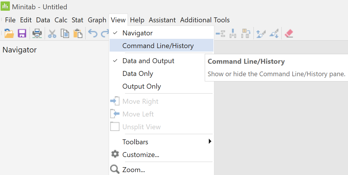
If the command pane is not visible, then on the main menu click 'View', then click on 'Command Line/History' The Command and History panes should then appear at the right edge of the Minitab window.

---




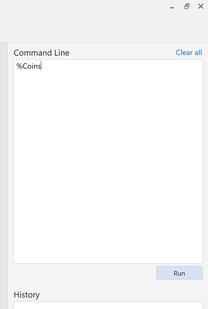
Click in the Command Line pane. Type % (the percentage symbol) followed immediately by the macro name (and its path if not in the default directory). You can omit the .mac extension. Just below the Command Line pane, click on 'Run'.

---




After a few seconds, results appear in the data and output panes. In the data pane, the entries in column 2 are '0' if that coin is a tail and '1' if that coin is a head. Column 3 keeps track of the relative frequency of heads so far.

---




The output pane includes the empirical probability (which will usually change with each run of this macro and is seldom exactly 0.5 but usually within 0.45 to 0.55).

---




The output pane also includes a time series chart.


---

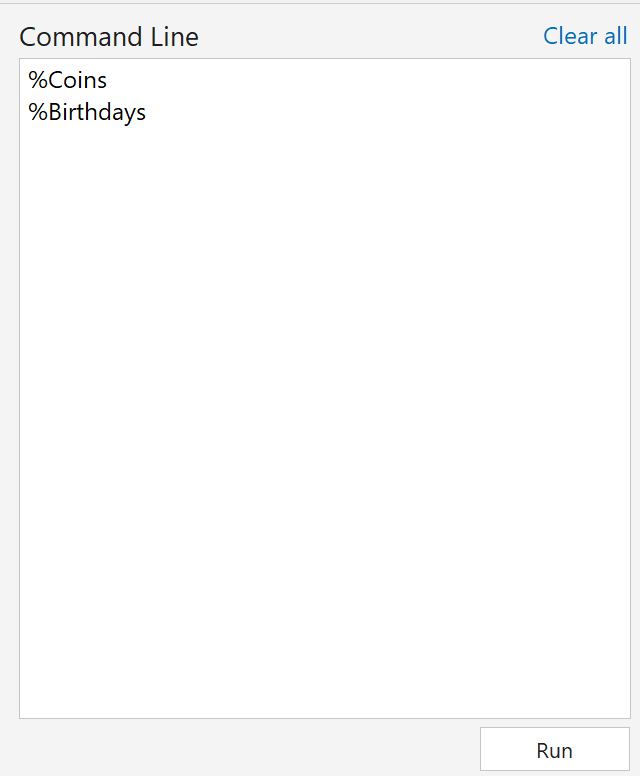
The power of the macro becomes apparent when we wish to repeat this simulation.
All that you need to do now is to click 'Run' just below the Command Line pane again and a new set of results appears in a new tab of the output pane.


You can export the above results into an .rtf file.
Then save your work and exit (or continue with the next simulation).

Simulation Example #3 - Shared Birthdays

The next example of the simulation of empirical probability is the famous “birthday problem”:   If n randomly chosen people are in a room, then what is the probability that at least two of them will share the same birthday?

Creation of a Macro File

Copy the following block of text and paste it into a blank document in a word processor (even Notepad will suffice).

---

gmacro
Birthdays
### Simulation to estimate the probability that at least two of (k1) people
### in a room will share a birthday.   The lowest (k1) for which the exact 
### probability exceeds 1/2 is k1 = 23 .
### Macro created 2003 03 10 and last modified 2021 02 16 by G.H. George

### mtitle / endmtitle needed to keep all output in one output pane
mtitle "Common birthdays simulation"
  erase c1-c8           # needed to ensure clear space in the worksheet
### Constants:
### k1 = number of people in the room
### k2 = number of trials
### k3 = trial index number (loop counter)
### k4 = relative frequency of shared birthdays
### Columns:
  name c1 'birthdays'   # birthdays of the (k1) people in this trial
  name c2 'ranks'       # ranks of birthday data in this trial
  name c3 'no ties'     # ranks if no ties (1 to #people)
  name c4 'diff.'       # abs.diff. of ranks with and without ties in this trial
  name c5 'num.shared'  # number of duplicates found in each trial
  name c6 'shared?'     # = 1 if any duplicates found, 0 if none found, for each trial
  name c7 'num.people'  # temporary column for input of k1
  name c8 'num.trials'  # temporary column for input of k2

### Note that keyboard data entry must be into columns, not constants:
  note Enter number of people:
  set c7;
    file "terminal";
    nobs 1.
  copy c7 k1
  note Enter number of trials:
  set c8;
    file "terminal";
    nobs 1.
  copy c8 k2
### Place the first (k1) natural numbers into column c3:
  set c3
    1:k1
    end.

  do k3=1:k2        # conduct the k2 simulations
      random k1 c1;
        integer 1 365.  # assign random birthdays to the k1 people in this trial
      sort c1 c1    # sort the birthdays into ascending order
      rank c1 c2
      let c4=abs(c2-c3) # zero unless shared birthdays are present in this trial
      let c5(k3)=sum(c4)
  enddo

### Each entry of c6 is 1 (true) if the corresponding entry of c5 is positive, 
### 0 (false) otherwise:
  let c6=(c5>0)

  let k4=sum(c6)/k2
  note The estimated probability that at least two people share the same birthday is
  print k4
  note Compare this with the true probability 
  note p = 1 - (365! / {(365-Num.people)!*(365)^(Num.people)})
  note (approximately 0.507 for 23 people)
endmtitle
endmacro

---

Save the file as "Birthdays.mac".

If you have Minitab installed on your computer, then you can save the macro in your Minitab Macros directory, (on some computers, it is at
"C:/Program Files/Minitab/Minitab 19/English/Macros/"), with the name "Birthdays.mac".

Some Notes on This Macro

Most of the details of this macro are explained by inline comments in the listing above.   One feature deserves additional comment here:   the trick used to detect equal values in a column of data.

Use the "rank" command to create a column showing the ranks of all entries in the column of (birthdays sorted into ascending order).   The n ranks will be exactly the first n natural numbers, unless any ties exist (that is, shared birthdays).   The sum of the absolute differences between the corresponding entries in the ranks column (c2) and the column containing the first n natural numbers (c3) will be zero if there are no ties, but positive if there are one or more ties.   This part of the algorithm is implemented in the lines inside the do loop

      sort c1 c1    # sort the birthdays into ascending order
      rank c1 c2
      let c4=abs(c2-c3) # zero unless shared birthdays are present in this trial
      let c5(k3)=sum(c4)

Each entry in the column c6 represents the result of one simulation.   Its value is 1 if any ties were detected and 0 if not.   By adding up all entries in that column, the total frequency of shared birthdays is calculated.

Execution of the Macro File

As before,

Click in the Command Line pane. Type % (the percentage symbol) followed immediately by the macro name (and its path if not in the default directory). Just below the Command Line pane, click on 'Run'.

---

Immediately the first 8 columns of the worksheet data pane are cleared and a new alias is set for each column.



A data entry box appears in the centre of the output pane. Enter the number of people in the room, then click on 'Submit'.

---




Immediately another data entry box appears in the centre of the output pane. Enter the number of trials, then click on 'Submit'.

---




The results appear after a few seconds.
They will usually be slightly different with each run.



---

A major advantage of the macro is that you can repeat this long sequence of commands by simply invoking the macro again with a single click on the 'Run' button and entering values again for the number of people in each room and the number of rooms.



You can copy and paste the above results from the output pane into an .rtf file.
Then save your work and exit.

---

A JavaScript simulation is also available.

---